Introductory Video

• The Machine Learning course includes several programming assignments which you’ll need to finish to complete the course. The assignments require the Octave scientific computing language.




• Octave is a free, open-source application available for many platforms. It has a text interface and an experimental graphical one. Octave is distributed under the GNU Public License, which means that it is always free to download and distribute.




• Use Download to install Octave for windows. "Warning: Do not install Octave 4.0.0";




• Installing Octave on GNU/Linux : On Ubuntu, you can use: sudo apt-get update && sudo apt-get install octave. On Fedora, you can use: sudo yum install octave-forge

• Files included in this exercise can be downloaded here ⇒ : Download




•         
          
  ex3.m - Octave/MATLAB script that steps you through part 1
  ex3_nn.m - Octave/MATLAB script that steps you through part 2
  ex3data1.mat - Training set of hand-written digits
  ex3weights.mat - Initial weights for the neural network exercise
  displayData.m - Function to help visualize the dataset
  fmincg.m - Function minimization routine (similar to fminunc)
  sigmoid.m - Sigmoid function
  lrCostFunction.m - Logistic regression cost function
  oneVsAll.m - Train a one-vs-all multi-class classifier
  predictOneVsAll.m - Predict using a one-vs-all multi-class classifier
  predict.m - Neural network prediction function       
          
  




• Throughout the exercise, you will be using the scripts ex3.m and ex3_nn.m.




• These scripts set up the dataset for the problems and make calls to functions that you will write.




• You do not need to modify these scripts.




• You are only required to modify functions in other files, by following the instructions in this assignment.

• For this exercise, you will use logistic regression and neural networks to recognize handwritten digits (from 0 to 9).




• Automated handwritten digit recognition is widely used today - from recognizing zip codes (postal codes) on mail envelopes to recognizing amounts written on bank checks.




• This exercise will show you how the methods you’ve learned can be used for this classification task.




• In the first part of the exercise, you will extend your previous implemention of logistic regression and apply it to one-vs-all classification.

• You are given a data set in ex3data1.mat that contains 5000 training examples of handwritten digits.




• The .mat format means that that the data has been saved in a native Octave/MATLAB matrix format, instead of a text (ASCII) format like a csv-file.




• These matrices can be read directly into your program by using the load command.




• After loading, matrices of the correct dimensions and values will appear in your program’s memory.




• The matrix will already be named, so you do not need to assign names to them.




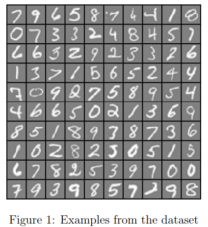
• % Load saved matrices from file
  load('ex3data1.mat');
  % The matrices X and y will now be in your Octave environment
  




• There are 5000 training examples in ex3data1.mat, where each training example is a 20 pixel by 20 pixel grayscale image of the digit.




• Each pixel is represented by a floating point number indicating the grayscale intensity at that location.




• The 20 by 20 grid of pixels is “unrolled” into a 400-dimensional vector. Each of these training examples becomes a single row in our data matrix X.




• This gives us a 5000 by 400 matrix X where every row is a training example for a handwritten digit image.




• 




• The second part of the training set is a 5000-dimensional vector y that contains labels for the training set.




• To make things more compatible with Octave/MATLAB indexing, where there is no zero index, we have mapped the digit zero to the value ten.




• Therefore, a "0" digit is labeled as "10", while the digits "1" to "9" are labeled as "1" to "9" in their natural order.

• You will begin by visualizing a subset of the training set.




• In Part 1 of ex3.m, the code randomly selects selects 100 rows from X and passes those rows to the displayData function.




• This function maps each row to a 20 pixel by 20 pixel grayscale image and displays the images together.




• We have provided the displayData function, and you are encouraged to examine the code to see how it works.




• After you run this step, you should see an image like Figure 1.




• 

• You will be using multiple one-vs-all logistic regression models to build a multi-class classifier.




• Since there are 10 classes, you will need to train 10 separate logistic regression classifiers.




• To make this training efficient, it is important to ensure that your code is well vectorized.




• In this section, you will implement a vectorized version of logistic regression that does not employ any for loops.




• You can use your code in the last exercise as a starting point for this exercise.




• We will begin by writing a vectorized version of the cost function. Recall that in (unregularized) logistic regression, the cost function is




• \( J(\theta) = - \frac{1}{m} \sum_{i=1}^m \large[ y^{(i)}\ \log (h_\theta (x^{(i)})) + (1 - y^{(i)})\ \log (1 - h_\theta(x^{(i)})) \)




• To compute each element in the summation, we have to compute \( h_\theta (x^{(i)} \) for every example i, where \( h_\theta (x^{(i)} = g(\theta^Tx^{(i)}) \) and \( g(z) = \frac{1}{1+e^{−z}} \) is the sigmoid function. It turns out that we can compute this quickly for all our examples by using matrix multiplication.




• Let us define X and θ as




• Then, by computing the matrix product \( X\theta \), we have




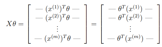
• In the last equality, we used the fact that \( a^Tb = b^Ta \) if a and b are vectors.




• This allows us to compute the products \( \theta^T x^{(i)} \) for all our examples i in one line of code.




• Your job is to write the unregularized cost function in the file lrCostFunction.m Your implementation should use the strategy we presented above to calculate \( \theta^T x^{(i)} \).




• You should also use a vectorized approach for the rest of the cost function.




• A fully vectorized version of lrCostFunction.m should not contain any loops.




• (Hint: You might want to use the element-wise multiplication operation (.*) and the sum operation sum when writing this function)

• When completed, this function is identical to your costFunctionReg() from ex2, but using vectorized methods.




• See the ex2 tutorials for the cost and gradient - they use vectorized methods.




• ex3.pdf tells you to first implement the unregularized parts, then to implement the regularized parts.




• Then you test your code, and then submit it for grading.




• Do not remove the line "grad = grad(:)" from the end of the lrCostFunction.m script template.




• This line guarantees that the grad value is returned as a column vector.

•  
   % input
  theta = [-2; -1; 1; 2];
  X = [ones(5,1) reshape(1:15,5,3)/10];
  y = [1;0;1;0;1] >= 0.5;       % creates a logical array
  
  % test the unregularized results
  [J grad] = lrCostFunction(theta, X, y, 0)
  
  % results
  J =  0.73482
  grad =
  
     0.146561
     0.051442
     0.124722
     0.198003
  
  % test the regularized results
  lambda = 3;
  [J grad] = lrCostFunction(theta, X, y, lambda)
  
  % results
  J =  2.5348
  grad =
  
     0.14656
    -0.54856
     0.72472
     1.39800   
      
      

• Recall that the gradient of the (unregularized) logistic regression cost is a vector where the jth element is defined as




• 




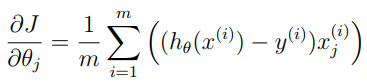
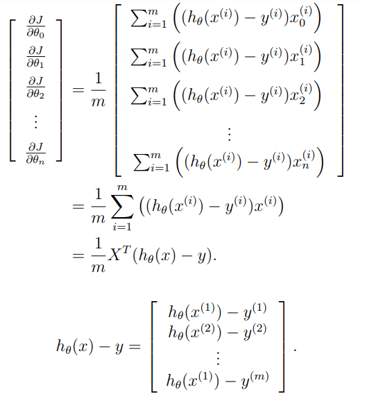
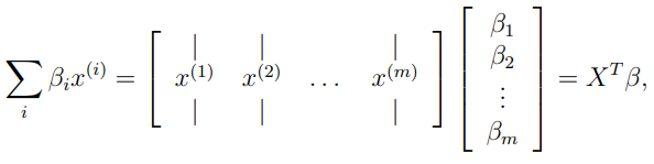
• where the values \( \beta_i = (h_\theta(x^{(i)}) − y^{(i)}) \)




• The expression above allows us to compute all the partial derivatives without any loops.




• If you are comfortable with linear algebra, we encourage you to work through the matrix multiplications above to convince yourself that the vectorized version does the same computations.




• You should now implement Equation 1 to compute the correct vectorized gradient.




• Once you are done, complete the function lrCostFunction.m by implementing the gradient




• Debugging Tip: Vectorizing code can sometimes be tricky.




• One common strategy for debugging is to print out the sizes of the matrices you are working with using the size function.




• For example, given a data matrix X of size 100 × 20 (100 examples, 20 features) and $\theta$, a vector with dimensions 20×1, you can observe that Xθ is a valid multiplication operation, while $\theta X$ is not.




• Furthermore, if you have a non-vectorized version of your code, you can compare the output of your vectorized code and non-vectorized code to make sure that they produce the same outputs.

• After you have implemented vectorization for logistic regression, you will now add regularization to the cost function.




• Recall that for regularized logistic regression, the cost function is defined as




• \( J(\theta) = - \frac{1}{m} \sum_{i=1}^m [ y^{(i)}\ \log (h_\theta (x^{(i)})) + (1 - y^{(i)})\ \log (1 - h_\theta(x^{(i)}))] + \frac{\lambda}{2m}\sum_{j=1}^n \theta_j^2 \)




• Note that you should not be regularizing $\theta_0$ which is used for the bias term.




• Correspondingly, the partial derivative of regularized logistic regression cost for $\theta_j$ is defined as




• 




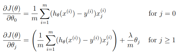
• Now modify your code in lrCostFunction to account for regularization. Once again, you should not put any loops into your code.




• Octave/MATLAB Tip: When implementing the vectorization for regularized logistic regression, you might often want to only sum and update certain elements of θ.




• In Octave/MATLAB, you can index into the matrices to access and update only certain elements. For example, A(:, 3:5) = B(:, 1:3) will replaces the columns 3 to 5 of A with the columns 1 to 3 from B.




• One special keyword you can use in indexing is the end keyword in indexing. This allows us to select columns (or rows) until the end of the matrix. For example, A(:, 2:end) will only return elements from the 2nd to last column of A.




• Thus, you could use this together with the sum and .^ operations to compute the sum of only the elements you are interested in (e.g., sum(z(2:end).^2)).




• In the starter code, lrCostFunction.m, we have also provided hints on yet another possible method computing the regularized gradient.

• In this part of the exercise, you will implement one-vs-all classification by training multiple regularized logistic regression classifiers, one for each of the K classes in our dataset (Figure 1).




• In the handwritten digits dataset, K = 10, but your code should work for any value of K.




• You should now complete the code in oneVsAll.m to train one classifier for each class. In particular, your code should return all the classifier parameters in a matrix \( \theta \in R^{K×(N+1)} \) , where each row of \( \theta \) corresponds to the learned logistic regression parameters for one class.




• You can do this with a “for”-loop from 1 to K, training each classifier independently.




• Note that the y argument to this function is a vector of labels from 1 to 10, where we have mapped the digit “0” to the label 10 (to avoid confusions with indexing).




• When training the classifier for class \( k \in {1, ..., K} \), you will want a mdimensional vector of labels y, where \( y_j \in 0, 1 \) indicates whether the j-th training instance belongs to class k (\( y_j = 1 \) ), or if it belongs to a different class (\( y_j = 0 \) ).




• You may find logical arrays helpful for this task.




• Octave/MATLAB Tip: Logical arrays in Octave/MATLAB are arrays which contain binary (0 or 1) elements. In Octave/MATLAB, evaluating the expression a == b for a vector a (of size m×1) and scalar b will return a vector of the same size as a with ones at positions where the elements of a are equal to b and zeroes where they are different. To see how this works for yourself, try the following code in Octave/MATLAB:




• a = 1:10; % Create a and b
  b = 3;
  a == b % You should try different values of b here
  




• Furthermore, you will be using fmincg for this exercise (instead of fminunc). fmincg works similarly to fminunc, but is more more efficient for dealing with a large number of parameters.




• After you have correctly completed the code for oneVsAll.m, the script ex3.m will continue to use your oneVsAll function to train a multi-class classifier.

• all_theta is a matrix, where there is a row for each of the trained thetas. In the exercise example, there are 10 rows, of 401 elements each. You know this because that's how all_theta was initialized in line 15 of the script template.




• (note that the submit grader's test case doesn't have 401 elements or 10 rows - your function must work for any size data set - so use the "num_labels" variable).




• Each call to fmincg() returns a theta vector. Be sure you use the lambda value provided in the function header.




• You then need to copy that vector into a row of all_theta.




• The oneVsAll.m script template contains several Hints and a code example to guide your work.




• The "y == c" statement creates a vector of 0's and 1's for each value of 'c' as you iterate from 1 to num_labels. Those are the effective 'y' values that are used for training to detect each label.




• Type these commands in your workspace to see how to copy a vector into a matrix:




• Q = zeros(5,3)      % create a test matrix of all-zeros
  v = [1 2 3]'        % create a column vector
  Q(2,:) = v          % copy v into the 2nd row of Q
  




• The syntax "(2,:)" means "use all columns of the 2nd row".

• %input:
  X = [magic(3) ; sin(1:3); cos(1:3)];
  y = [1; 2; 2; 1; 3];
  num_labels = 3;
  lambda = 0.1;
  [all_theta] = oneVsAll(X, y, num_labels, lambda)
  %output:
  all_theta =
    -0.559478   0.619220  -0.550361  -0.093502
    -5.472920  -0.471565   1.261046   0.634767
     0.068368  -0.375582  -1.652262  -1.410138
      

• After training your one-vs-all classifier, you can now use it to predict the digit contained in a given image.




• For each input, you should compute the “probability” that it belongs to each class using the trained logistic regression classifiers.




• Your one-vs-all prediction function will pick the class for which the corresponding logistic regression classifier outputs the highest probability and return the class label (1, 2,..., or K) as the prediction for the input example.




• You should now complete the code in predictOneVsAll.m to use the one-vs-all classifier to make predictions.




• Once you are done, ex3.m will call your predictOneVsAll function using the learned value of \( \theta \). You should see that the training set accuracy is about 94.9% (i.e., it classifies 94.9% of the examples in the training set correctly).

• The code you add to predictOneVsAll.m can be as little as two lines:




• one line to calculate the sigmoid() of the product of X and all_theta. X is (m x n), and all_theta is (num_labels x n), so you'll need a transposition to get a result of (m x num_labels)




• one line to return the classifier which has the max value. The size will be (m x 1). Use the "help max" command in your workspace to learn how the max() function returns two values.




• Note that your function must return the predictions as a column vector - size (m x 1). If you return a row vector, the script will not compute the accuracy correctly.

•  % input:
  all_theta = [1 -6 3; -2 4 -3];
  X = [1 7; 4 5; 7 8; 1 4];
  predictOneVsAll(all_theta, X)
  %output:
  ans =
     1
     2
     2
     1   
      
      

• In the previous part of this exercise, you implemented multi-class logistic regression to recognize handwritten digits.




• However, logistic regression cannot form more complex hypotheses as it is only a linear classifier.




• In this part of the exercise, you will implement a neural network to recognize handwritten digits using the same training set as before.




• The neural network will be able to represent complex models that form non-linear hypotheses.




• For this , you will be using parameters from a neural network that we have already trained. Your goal is to implement the feedforward propagation algorithm to use our weights for prediction.




• In next exercise, you will write the backpropagation algorithm for learning the neural network parameters.




• The provided script, ex3 nn.m, will help you step through this exercise.

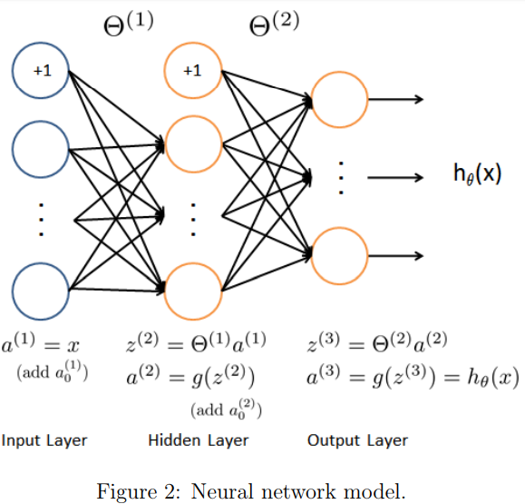
• Our neural network is shown in Figure 2. It has 3 layers – an input layer, a hidden layer and an output layer.




• Recall that our inputs are pixel values of digit images.




• Since the images are of size 20×20, this gives us 400 input layer units (excluding the extra bias unit which always outputs +1).




• As before, the training data will be loaded into the variables X and y. You have been provided with a set of network parameters \( \theta^{(1)}, \theta^{(2)}\) already trained by us.




• These are stored in ex3weights.mat and will be loaded by ex3_nn.m into Theta1 and Theta2 The parameters have dimensions that are sized for a neural network with 25 units in the second layer and 10 output units (corresponding to the 10 digit classes).




• % Load saved matrices from file
  load('ex3weights.mat');
  % The matrices Theta1 and Theta2 will now be in your Octave
  % environment
  % Theta1 has size 25 x 401
  % Theta2 has size 10 x 26
  




• You could add more features (such as polynomial features) to logistic regression, but that can be very expensive to train.




• 

• Now you will implement feedforward propagation for the neural network. You will need to complete the code in predict.m to return the neural network’s prediction.




• You should implement the feedforward computation that computes \( h_\theta(x^{(i)})\) for every example i and returns the associated predictions.




• Similar to the one-vs-all classification strategy, the prediction from the neural network will be the label that has the largest output \( (h_\theta(x))_k \).




• Implementation Note: The matrix X contains the examples in rows. When you complete the code in predict.m, you will need to add the column of 1’s to the matrix.




• The matrices Theta1 and Theta2 contain the parameters for each unit in rows. Specifically, the first row of Theta1 corresponds to the first hidden unit in the second layer.




• In Octave/MATLAB, when you compute \(z^{(2)} = \theta^{(1)}a^{(1)}\), be sure that you index (and if necessary, transpose) X correctly so that you get \( a^{(l)} \) as a column vector.




• Once you are done, ex3 nn.m will call your predict function using the loaded set of parameters for Theta1 and Theta2.




• You should see that the accuracy is about 97.5%. After that, an interactive sequence will launch displaying images from the training set one at a time, while the console prints out the predicted label for the displayed image. To stop the image sequence, press Ctrl-C.

• Here is an outline for forward propagation using the vectorized method. This is an implementation of the formula in Figure 2 on Page 11 of ex3.pdf.




• Add a column of 1's to X (the first column), and it becomes 'a1'.




• Multiply by Theta1 and you have 'z2'.




• Compute the sigmoid() of 'z2', then add a column of 1's, and it becomes 'a2' Multiply by Theta2, compute the sigmoid() and it becomes 'a3'.




• Now use the max(a3, [], 2) function to return two vectors - one of the highest value for each row, and one with its index. Ignore the highest values. Keep the vector of the indexes where the highest values were found. These are your predictions.




• Note: When you multiply by the Theta matrices, you'll have to use transposition to get a result that is the correct size.




• Note: The predictions must be returned as a column vector - size (m x 1). If you return a row vector, the script will not compute the accuracy correctly.




• Note: Not getting the correct results? In the hidden layer, be sure you use sigmoid() first, then add the bias unit.




• ------ dimensions of the variables ---------
  
  a1 is (m x n), where 'n' is the number of features including the bias unit
  
  Theta1 is (h x n) where 'h' is the number of hidden units
  
  a2 is (m x (h + 1))
  
  Theta2 is (c x (h + 1)), where 'c' is the number of labels.
  
  a3 is (m x c)
  
  p is a vector of size (m x 1)
  
  

• Theta1 = reshape(sin(0 : 0.5 : 5.9), 4, 3);
  Theta2 = reshape(sin(0 : 0.3 : 5.9), 4, 5);
  X = reshape(sin(1:16), 8, 2);
  p = predict(Theta1, Theta2, X)
  % you should see this result
  p = 
    4
    1
    1
    4
    4
    4
    4
    2
    
    
  Here are the values for the "a3" layer in the test case for predict()
  
  a3 =
  
     0.53036   0.54588   0.55725   0.56352
     0.54459   0.54298   0.53754   0.52875
     0.49979   0.49616   0.49288   0.49024
     0.41357   0.42199   0.43736   0.45844
     0.37321   0.40368   0.44349   0.48911
     0.42073   0.45935   0.50210   0.54464
     0.50962   0.53216   0.55173   0.56659
     0.54882   0.55033   0.54738   0.54021