Setting Up Your Programming Assignment Environment
Introductory Video
The Machine Learning course includes several programming assignments which you’ll need to finish to complete the course. The assignments require the Octave scientific computing language.
Octave is a free, open-source application available for many platforms. It has a text interface and an experimental graphical one. Octave is distributed under the GNU Public License, which means that it is always free to download and distribute.
Use Download to install Octave for windows. "Warning: Do not install Octave 4.0.0";
Installing Octave on GNU/Linux : On Ubuntu, you can use: sudo apt-get update && sudo apt-get install octave. On Fedora, you can use: sudo yum install octave-forge
Programming Exercise 4: Neural Networks Learning
Files included in this exercise can be downloaded here ⇒ : Download
Files included in this exercise :

ex4.m - Octave/MATLAB script that steps you through the exercise
ex4data1.mat - Training set of hand-written digits
ex4weights.mat - Neural network parameters for exercise 4
submit.m - Submission script that sends your solutions to our servers
displayData.m - Function to help visualize the dataset
fmincg.m - Function minimization routine (similar to fminunc)
sigmoid.m - Sigmoid function
computeNumericalGradient.m - Numerically compute gradients
checkNNGradients.m - Function to help check your gradients
debugInitializeWeights.m - Function for initializing weights
predict.m - Neural network prediction function
sigmoidGradient.m - Compute the gradient of the sigmoid function
randInitializeWeights.m - Randomly initialize weights
nnCostFunction.m - Neural network cost function
Throughout the exercise, you will be using the script ex4.m. These scripts set up the dataset for the problems and make calls to functions that you will write. You do not need to modify the script. You are only required to modify functions in other files, by following the instructions in this assignment.
Neural Networks
In the previous exercise, you implemented feedforward propagation for neural networks and used it to predict handwritten digits with the weights we provided.
In this exercise, you will implement the backpropagation algorithm to learn the parameters for the neural network.
The provided script, ex4.m, will help you step through this exercise.
Step 1: Visualizing the data
In the first part of ex4.m, the code will load the data and display it on a 2-dimensional plot (Figure 1) by calling the function displayData.
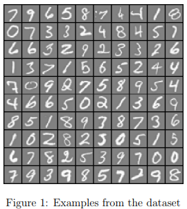
This is the same dataset that you used in the previous exercise. There are 5000 training examples in ex3data1.mat, where each training example is a 20 pixel by 20 pixel grayscale image of the digit.
Each pixel is represented by a floating point number indicating the grayscale intensity at that location. The 20 by 20 grid of pixels is “unrolled” into a 400-dimensional vector.
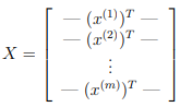
Each of these training examples becomes a single row in our data matrix X.
This gives us a 5000 by 400 matrix X where every row is a training example for a handwritten digit image.
The second part of the training set is a 5000-dimensional vector y that contains labels for the training set.
To make things more compatible with Octave/MATLAB indexing, where there is no zero index, we have mapped the digit zero to the value ten. Therefore, a '0' digit is labeled as '10', while the digits '1' to '9' are labeled as '1' to '9' in their natural order.
Step 2: Model representation
Our neural network is shown in Figure 2.
It has 3 layers – an input layer, a hidden layer and an output layer. Recall that our inputs are pixel values of digit images.
Since the images are of size 20 × 20, this gives us 400 input layer units (not counting the extra bias unit which always outputs +1). The training data will be loaded into the variables X and y by the ex4.m script.
You have been provided with a set of network parameters (Θ(1), Θ(2)) already trained by us.
These are stored in ex4weights.mat and will be loaded by ex4.m into Theta1 and Theta2.
The parameters have dimensions that are sized for a neural network with 25 units in the second layer and 10 output units (corresponding to the 10 digit classes).
% Load saved matrices from file
load('ex4weights.mat');
% The matrices Theta1 and Theta2 will now be in your workspace
% Theta1 has size 25 x 401
% Theta2 has size 10 x 26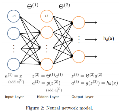
Step 3 : Feedforward and cost function
Now you will implement the cost function and gradient for the neural network. First, complete the code in nnCostFunction.m to return the cost.
Recall that the cost function for the neural network (without regularization) is
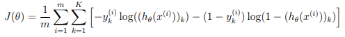
where \( h_\theta(x^{(i)}) \) is computed as shown in the Figure 2 and K = 10 is the total number of possible labels.
Note that \( h_\theta(x^{(i)})_k = a^{(3)}_k \) is the activation (output value) of the k-th output unit.
Also, recall that whereas the original labels (in the variable y) were 1, 2, ..., 10, for the purpose of training a neural network, we need to recode the labels as vectors containing only values 0 or 1, so that
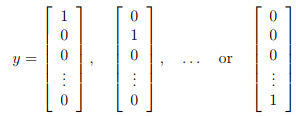
For example, if \( x^{(i)} \) is an image of the digit 5, then the corresponding \( y^{(i)} \) (that you should use with the cost function) should be a 10-dimensional vector with \( y_5 = 1 \), and the other elements equal to 0.
You should implement the feedforward computation that computes \( h_\theta(x^{(i)}) \) for every example i and sum the cost over all examples.
Your code should also work for a dataset of any size, with any number of labels (you can assume that there are always at least K ≥ 3 labels).
Implementation Note: The matrix X contains the examples in rows (i.e., X(i,:)’ is the i-th training example \( x^{(i)} \) , expressed as a n × 1 vector.)
When you complete the code in nnCostFunction.m, you will need to add the column of 1’s to the X matrix.
The parameters for each unit in the neural network is represented in Theta1 and Theta2 as one row. Specifically, the first row of Theta1 corresponds to the first hidden unit in the second layer.
You can use a for-loop over the examples to compute the cost.
Once you are done, ex4.m will call your nnCostFunction using the loaded set of parameters for Theta1 and Theta2. You should see that the cost is about 0.287629.
ex4 Tutorial for forward propagation and cost
Each of these variables will have a subscript, noting which NN layer it is associated with.
\( \Theta \): A Theta matrix of weights to compute the inner values of the neural network. When we used a vector theta, it was noted with the lower-case theta character \( \theta \)
z : is the result of multiplying a data vector with a \( \Theta \) matrix. A typical variable name would be "z2".
a : The "activation" output from a neural layer. This is always generated using a sigmoid function g() on a z value. A typical variable name would be "a2".
\( \delta \) : lower-case delta is used for the "error" term in each layer. A typical variable name would be "d2".
\( \Delta \) : upper-case delta is used to hold the sum of the product of a \( \delta \) value with the previous layer's a value. In the vectorized solution, these sums are calculated automatically though the magic of matrix algebra. A typical variable name would be "Delta2".
\( \Theta_{gradient} \) : This is the thing we're solving for, the partial derivative of theta. There is one of these variables associated with each \( \Delta \). These values are returned by nnCostFunction(), so the variable names must be "Theta1_grad" and "Theta2_grad".
g() is the sigmoid function.
g'() is the sigmoid gradient function.
Tip: One handy method for excluding a column of bias units is to use the notation SomeMatrix(:,2:end). This selects all of the rows of a matrix, and omits the entire first column.
See the Appendix below for information on the sizes of the data objects.
Appendix:

Here are the sizes for the Ex4 character recognition example, using the method described in this tutorial.

NOTE: The submit grader (and the gradient checking process) uses a different test case; these sizes are NOT for the submit grader or for gradient checking.

a1: 5000x401

z2: 5000x25

a2: 5000x26

a3: 5000x10

d3: 5000x10

d2: 5000x25

Theta1, Delta1 and Theta1_grad: 25x401

Theta2, Delta2 and Theta2_grad: 10x26
A note regarding bias units, regularization, and back-propagation:
There are two methods for handing exclusion of the bias units in the Theta matrices in the back-propagation and gradient calculations. I've described only one of them here, it's the one that I understood the best. Both methods work, choose the one that makes sense to you and avoids dimension errors. It matters not a whit whether the bias unit is excluded before or after it is calculated - both methods give the same results, though the order of operations and transpositions required may be different. Those with contrary opinions are welcome to write their own tutorial.
Forward Propagation:
We'll start by outlining the forward propagation process. Though this was already accomplished once during Exercise 3, you'll need to duplicate some of that work because computing the gradients requires some of the intermediate results from forward propagation. Also, the y values in ex4 are a matrix, instead of a vector. This changes the method for computing the cost J.
Expand the 'y' output values into a matrix of single values. This is most easily done using an eye() matrix of size num_labels, with vectorized indexing by 'y'. A useful variable name would be "y_matrix", as this...
y_matrix = eye(num_labels)(y,:)
Note: For MATLAB users, this expression must be split into two lines, such as.
eye_matrix = eye(num_labels)
y_matrix = eye_matrix(y,:)
Perform the forward propagation:
\( a_1 \) equals the X input matrix with a column of 1's added (bias units) as the first column.
\( z_2 \) equals the product of \( a_1 \) and \( \Theta_1 , a_2 \) is the result of passing \( z_2 \) through g().
Then add a column of bias units to \( a_2 \) (as the first column).
NOTE: Be sure you DON'T add the bias units as a new row of Theta.
\( z_3 \) equals the product of \( a_2 \) and \( \Theta_2 \)
\( a_3 \) is the result of passing \( z_3 \) through g()
Cost Function, non-regularized: - Compute the unregularized cost using \( a_3 \) , your y_matrix, and m (the number of training examples). Note that the 'h' argument inside the log() function is exactly a3. Cost should be a scalar value. Since y_matrix and a3 are both matrices, you need to compute the double-sum. Remember to use element-wise multiplication with the log() function.
Also, we're using the natural log, not log10().
Now you can run ex4.m to check the unregularized cost is correct, then you can submit this portion to the grader.
Step 4 : Regularized cost function
The cost function for neural networks with regularization is given by
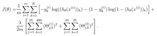
You can assume that the neural network will only have 3 layers – an input layer, a hidden layer and an output layer.
However, your code should work for any number of input units, hidden units and outputs units. While we have explicitly listed the indices above for \( Θ^{(1)} \) and \( Θ^{(2)} \) for clarity, do note that your code should in general work with \( Θ^{(1)} \) and \( Θ^{(2)} \) of any size.
Note that you should not be regularizing the terms that correspond to the bias. For the matrices Theta1 and Theta2, this corresponds to the first column of each matrix.
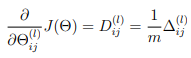
You should now add regularization to your cost function. Notice that you can first compute the unregularized cost function J using your existing nnCostFunction.m and then later add the cost for the regularization terms.
Once you are done, ex4.m will call your nnCostFunction using the loaded set of parameters for Theta1 and Theta2, and λ = 1.
You should see that the cost is about 0.383770.
Backpropagation
In this part of the exercise, you will implement the backpropagation algorithm to compute the gradient for the neural network cost function.
You will need to complete the nnCostFunction.m so that it returns an appropriate value for grad.
Once you have computed the gradient, you will be able to train the neural network by minimizing the cost function J(Θ) using an advanced optimizer such as fmincg.
You will first implement the backpropagation algorithm to compute the gradients for the parameters for the (unregularized) neural network.
After you have verified that your gradient computation for the unregularized case is correct, you will implement the gradient for the regularized neural network.
Sigmoid gradient
To help you get started with this part of the exercise, you will first implement the sigmoid gradient function.
The gradient for the sigmoid function can be computed as
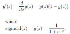
When you are done, try testing a few values by calling sigmoidGradient(z) at the Octave/MATLAB command line.
For large values (both positive and negative) of z, the gradient should be close to 0.
When z = 0, the gradient should be exactly 0.25.
Your code should also work with vectors and matrices.
For a matrix, your function should perform the sigmoid gradient function on every element.
ex4 test case for sigmoidGradient()
sigmoidGradient([[-1 -2 -3] ; magic(3)])
ans =
  1.9661e-001  1.0499e-001  4.5177e-002
  3.3524e-004  1.9661e-001  2.4665e-003
  4.5177e-002  6.6481e-003  9.1022e-004
  1.7663e-002  1.2338e-004  1.0499e-001
Random initialization
When training neural networks, it is important to randomly initialize the parameters for symmetry breaking.
One effective strategy for random initialization is to randomly select values for Θ(l) uniformly in the range \( [−\epsilon_{init}, \epsilon_{init}] \).
You should use \( \epsilon_{init} \) = 0.12. This range of values ensures that the parameters are kept small and makes the learning more efficient.
Your job is to complete randInitializeWeights.m to initialize the weights for Θ; modify the file and fill in the following code:
% Randomly initialize the weights to small values
epsilon_init = 0.12;
W = rand(L_out, 1 + L_in) * 2 * epsilon_init − epsilon_init;
Backpropagation
 Now, you will implement the backpropagation algorithm. Recall that
the intuition behind the backpropagation algorithm is as follows.
Now, you will implement the backpropagation algorithm. Recall that
the intuition behind the backpropagation algorithm is as follows. Given a training example \( (x^{(t)}, y^{(t)}) \), we will first run a “forward pass” to compute all the activations throughout the network, including the output value of the hypothesis \( h_\theta(x) \).
Then, for each node j in layer l, we would like to compute an “error term” \( \delta_j^{(l)} \) that measures how much that node was “responsible” for any errors in our output.
For an output node, we can directly measure the difference between the network’s activation and the true target value, and use that to define \( \delta_j^{(3)} \) (since layer 3 is the output layer).
For the hidden units, you will compute \( \delta_j^{(l)} \) based on a weighted average of the error terms of the nodes in layer (l + 1).
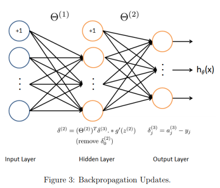
In detail, here is the backpropagation algorithm (also depicted in Figure 3).
You should implement steps 1 to 4 in a loop that processes one example at a time.
Concretely, you should implement a for-loop for t = 1:m and place steps 1-4 below inside the for-loop, with the t th iteration performing the calculation on the t th training example \( (x^{(t)}, y^{(t)}) \).
Step 5 will divide the accumulated gradients by m to obtain the gradients for the neural network cost function.
Set the input layer’s values \( (a^{(1)}) \) to the t-th training example \( x^{(t)} \). Perform a feedforward pass (Figure 2), computing the activations \( (z^{(2)}, a^{(2)}, z^{(3)}, a^{(3)} ) \) for layers 2 and 3.
Note that you need to add a +1 term to ensure that the vectors of activations for layers \( a^{(1)} \) and \( a^{(2)} \) also include the bias unit.
In Octave/MATLAB, if a 1 is a column vector, adding one corresponds to a_1 = [1 ; a_1].
For each output unit k in layer 3 (the output layer), set \( \delta_k^{(3)} = (a_k^{(3)} - y_k) \) where \( y_k \in {0, 1} \) indicates whether the current training example belongs to class k (\( y_k = 1 \) ), or if it belongs to a different class ( \( y_k = 0 \) ).
You may find logical arrays helpful for this task (explained in the previous programming exercise).
For the hidden layer l = 2, set \( \delta^{(2)} = (\theta^{(2)})^T \delta^{(3)} .* g'(z^{(2)}) \)
Accumulate the gradient from this example using the following formula. Note that you should skip or remove \( \delta_0^{(2)} \) .
In Octave/MATLAB, removing \( \delta_0^{(2)} \) corresponds to delta_2 = delta_2(2:end) \( \Delta^{(l)} := \Delta^{(l)} + \delta^{(l+1)}(a^{(l)})^T \)
Obtain the (unregularized) gradient for the neural network cost function by dividing the accumulated gradients by 1/m :
Octave/MATLAB Tip: You should implement the backpropagation algorithm only after you have successfully completed the feedforward and cost functions. While implementing the backpropagation algorithm, it is often useful to use the size function to print out the sizes of the variables you are working with if you run into dimension mismatch errors (“nonconformant arguments” errors in Octave/MATLAB
After you have implemented the backpropagation algorithm, the script ex4.m will proceed to run gradient checking on your implementation. The gradient check will allow you to increase your confidence that your code is computing the gradients correctly.
ex4 tutorial for nnCostFunction and backpropagation
Let:

m = the number of training examples

n = the number of training features, including the initial bias unit.

h = the number of units in the hidden layer - NOT including the bias unit

r = the number of output classifications
Step 1: Perform forward propagation, see the separate tutorial if necessary.
Step 2: \( \delta_3 \) or d3 is the difference between a3 and the y_matrix. The dimensions are the same as both, (m x r).
Step 3: z2 comes from the forward propagation process - it's the product of a1 and Theta1, prior to applying the sigmoid() function. Dimensions are (m x n) \cdot⋅ (n x h) --> (m x h). In step 4, you're going to need the sigmoid gradient of z2. We know that if u = sigmoid(z2), then sigmoidGradient(z2) = u .* (1-u).
Step 4: \( \delta_2 \) or d2 is tricky. It uses the (:,2:end) columns of Theta2. d2 is the product of d3 and Theta2 (without the first column), then multiplied element-wise by the sigmoid gradient of z2. The size is \( (m x r) \cdot⋅ (r x h) --> (m x h) \) . The size is the same as z2.
Note: Excluding the first column of Theta2 is because the hidden layer bias unit has no connection to the input layer - so we do not use backpropagation for it. See Figure 3 in ex4.pdf for a diagram showing this.
Step 5: \( \Delta_1 \) or Delta1 is the product of d2 and a1. The size is \( (h x m) \cdot⋅ (m x n) --> (h x n) \)
Step 6: \( \Delta_2 \) or Delta2 is the product of d3 and a2. The size is \( (r x m) \cdot⋅ (m x [h+1]) --> (r x [h+1]) \)
Step 7: Theta1_grad and Theta2_grad are the same size as their respective Deltas, just scaled by 1/m.
Now you have the unregularized gradients. Check your results using ex4.m using test cases mentioned below.
Gradient checking
In your neural network, you are minimizing the cost function J(Θ). To perform gradient checking on your parameters, you can imagine “unrolling” the parameters \( Θ^{(1)}, Θ^{(2)} \) into a long vector θ.
By doing so, you can think of the cost function being J(θ) instead and use the following gradient checking procedure.
Suppose you have a function \( f_i(θ) \) that purportedly computes \( \frac{\partial}{\partial \theta_i} J(θ); \) you’d like to check if \( f_i \) is outputting correct derivative values.
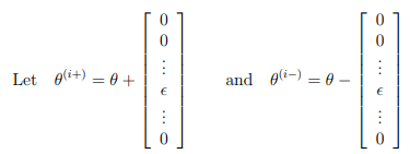
So, \( θ^{(i+)} \) is the same as θ, except its i-th element has been incremented by \( \epsilon \).
Similarly, \( θ^{(i-)} \) is the corresponding vector with the i-th element decreased by \( \epsilon \). You can now numerically verify fi(θ)’s correctness by checking, for each i, that:
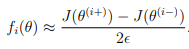
The degree to which these two values should approximate each other will depend on the details of J.
But assuming \( \epsilon = 10^{−4} \) , you’ll usually find that the left- and right-hand sides of the above will agree to at least 4 significant digits (and often many more).
We have implemented the function to compute the numerical gradient for you in computeNumericalGradient.m. While you are not required to modify the file, we highly encourage you to take a look at the code to understand how it works.
In the next step of ex4.m, it will run the provided function checkNNGradients.m which will create a small neural network and dataset that will be used for checking your gradients. If your backpropagation implementation is correct, you should see a relative difference that is less than 1e-9.
Practical Tip: When performing gradient checking, it is much more efficient to use a small neural network with a relatively small number of input units and hidden units, thus having a relatively small number of parameters. Each dimension of θ requires two evaluations of the cost function and this can be expensive. In the function checkNNGradients, our code creates a small random model and dataset which is used with computeNumericalGradient for gradient checking. Furthermore, after you are confident that your gradient computations are correct, you should turn off gradient checking before running your learning algorithm.
Practical Tip: Gradient checking works for any function where you are computing the cost and the gradient. Concretely, you can use the same computeNumericalGradient.m function to check if your gradient implementations for the other exercises are correct too (e.g., logistic regression’s cost function).
Regularized Neural Networks
After you have successfully implemeted the backpropagation algorithm, you will add regularization to the gradient. To account for regularization, it turns out that you can add this as an additional term after computing the gradients using backpropagation.
Specifically, after you have computed \( \Delta^{(l)}_{i,j} \) using backpropagation, you should add regularization using
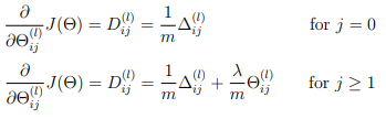
Note that you should not be regularizing the first column of \( Θ^{(l)} \) which is used for the bias term. Furthermore, in the parameters \( Θ^{(l)}_{ij} \) , i is indexed starting from 1, and j is indexed starting from 0. Thus,
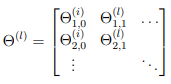
Somewhat confusingly, indexing in Octave/MATLAB starts from 1 (for both i and j), thus Theta1(2, 1) actually corresponds to \( Θ^{(l)}_{2,0} \) (i.e., the entry in the second row, first column of the matrix Θ(1) shown above) Now modify your code that computes grad in nnCostFunction to account for regularization.
After you are done, the ex4.m script will proceed to run gradient checking on your implementation.
If your code is correct, you should expect to see a relative difference that is less than 1e-9.
===== Regularization of the gradient =========== (Steps 1- 7 should be completed previously)
Since Theta1 and Theta2 are local copies, and we've already computed our hypothesis value during forward-propagation, we're free to modify them to make the gradient regularization easy to compute.
Step 8: So, set the first column of Theta1 and Theta2 to all-zeros. Here's a method you can try in your workspace console:
Step 9: Scale each Theta matrix by \( \lambda/m \) . Use enough parenthesis so the operation is correct.
Step 10: Add each of these modified-and-scaled Theta matrices to the un-regularized Theta gradients that you computed earlier.
You're done. Use the test case (from the Resources menu) to test your code, and the ex4 script, then run the submit script.
The additional Test Case for ex4 includes the values of the internal variables discussed in the tutorial.
Appendix:

Here are the sizes for the Ex4 digit recognition example, using the method described in this tutorial.


a1: 5000x401

z2: 5000x25

a2: 5000x26

a3: 5000x10

d3: 5000x10

d2: 5000x25

Theta1, Delta1 and Theta1_grad: 25x401

Theta2, Delta2 and Theta2_grad: 10x26
Test cases for ex4 nnCostFunction()
[J grad] = nnCostFunction(nn, il, hl, nl, X, y, 0)
J =  7.4070
grad =
   0.766138
   0.979897
  -0.027540
  -0.035844
  -0.024929
  -0.053862
   0.883417
   0.568762
   0.584668
   0.598139
   0.459314
   0.344618
   0.256313
   0.311885
   0.478337
   0.368920
   0.259771
   0.322331

Delta1 =
  2.298 -0.082 -0.074
  2.939 -0.107 -0.161

Delta2 =
  2.650  1.377  1.435
  1.706  1.033  1.106
  1.754  0.768  0.779
  1.794  0.935  0.966

a2 =
   1.00000   0.51350   0.54151
   1.00000   0.37196   0.35705
   1.00000   0.66042   0.70880

a3 =
   0.88866   0.90743   0.92330   0.93665
   0.83818   0.86028   0.87980   0.89692
   0.92341   0.93858   0.95090   0.96085

d3 =
   0.888659   0.907427   0.923305  -0.063351
   0.838178  -0.139718   0.879800   0.896918
   0.923414   0.938578  -0.049102   0.960851

d2 =
   0.79393   1.05281
   0.73674   0.95128
   0.76775   0.93560

Delta1/m =
   0.766138  -0.027540  -0.024929
   0.979897  -0.035844  -0.053862

Delta2/m =
   0.88342   0.45931   0.47834
   0.56876   0.34462   0.36892
   0.58467   0.25631   0.25977
   0.59814   0.31189   0.32233
Test Case with regularization
il = 2;              % input layer
hl = 2;              % hidden layer
nl = 4;              % number of labels
nn = [ 1:18 ] / 10;  % nn_params
X = cos([1 2 ; 3 4 ; 5 6]);
y = [4; 2; 3];
lambda = 4;
[J grad] = nnCostFunction(nn, il, hl, nl, X, y, lamb

J = 19.474
grad =
0.76614
0.97990
0.37246
0.49749
0.64174
0.74614
0.88342
0.56876
0.58467
0.59814
1.92598
1.94462
1.98965
2.17855
2.47834
2.50225
2.52644
2.72233

d2 =
   0.79393   1.05281
   0.73674   0.95128
   0.76775   0.93560

d3 =
   0.888659   0.907427   0.923305  -0.063351
   0.838178  -0.139718   0.879800   0.896918
   0.923414   0.938578  -0.049102   0.960851

Delta1 =
   2.298415  -0.082619  -0.074786
   2.939691  -0.107533  -0.161585

Delta2 =
   2.65025   1.37794   1.43501
   1.70629   1.03385   1.10676
   1.75400   0.76894   0.77931
   1.79442   0.93566   0.96699

z2 =
   0.054017   0.166433
  -0.523820  -0.588183
   0.665184   0.889567

sigmoidGradient(z2)
ans =
   0.24982   0.24828
   0.23361   0.22957
   0.22426   0.20640

a2 =
   1.00000   0.51350   0.54151
   1.00000   0.37196   0.35705
   1.00000   0.66042   0.70880

a3 =
   0.88866   0.90743   0.92330   0.93665
   0.83818   0.86028   0.87980   0.89692
   0.92341   0.93858   0.95090   0.96085
Learning parameters using fmincg
After you have successfully implemented the neural network cost function and gradient computation, the next step of the ex4.m script will use fmincg to learn a good set parameters.
After the training completes, the ex4.m script will proceed to report the training accuracy of your classifier by computing the percentage of examples it got correct.
If your implementation is correct, you should see a reported training accuracy of about 95.3% (this may vary by about 1% due to the random initialization).
It is possible to get higher training accuracies by training the neural network for more iterations.
We encourage you to try training the neural network for more iterations (e.g., set MaxIter to 400) and also vary the regularization parameter λ.
With the right learning settings, it is possible to get the neural network to perfectly fit the training set.
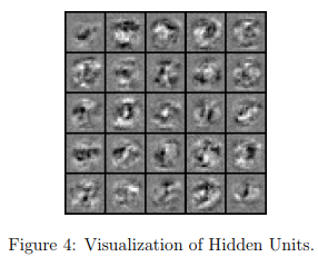
Visualizing the hidden layer
One way to understand what your neural network is learning is to visualize what the representations captured by the hidden units.
Informally, given a particular hidden unit, one way to visualize what it computes is to find an input x that will cause it to activate (that is, to have an activation value \(a_i^{(l)} \) close to 1).
For the neural network you trained, notice that the ith row of \( Θ^{(1)} \) is a 401-dimensional vector that represents the parameter for the ith hidden unit.
If we discard the bias term, we get a 400 dimensional vector that represents the weights from each input pixel to the hidden unit.
Thus, one way to visualize the “representation” captured by the hidden unit is to reshape this 400 dimensional vector into a 20 × 20 image and display it.
The next step of ex4.m does this by using the displayData function and it will show you an image (similar to Figure 4) with 25 units, each corresponding to one hidden unit in the network.
In your trained network, you should find that the hidden units corresponds roughly to detectors that look for strokes and other patterns in the input.