Setting Up Your Programming Assignment Environment
Introductory Video
The Machine Learning course includes several programming assignments which you’ll need to finish to complete the course. The assignments require the Octave scientific computing language.
Octave is a free, open-source application available for many platforms. It has a text interface and an experimental graphical one. Octave is distributed under the GNU Public License, which means that it is always free to download and distribute.
Use Download to install Octave for windows. "Warning: Do not install Octave 4.0.0";
Installing Octave on GNU/Linux : On Ubuntu, you can use: sudo apt-get update && sudo apt-get install octave. On Fedora, you can use: sudo yum install octave-forge
Introduction
In this exercise, you will implement regularized linear regression and use it to study models with different bias-variance properties.
Files included in this exercise can be downloaded here ⇒ : Download
If needed, use the cd command in Octave/MATLAB to change to this directory before starting this exercise.
You can also find instructions for installing Octave/MATLAB above
ex5.m - Octave/MATLAB script that steps you through the exercise
ex5data1.mat - Dataset
submit.m - Submission script that sends your solutions to our servers
featureNormalize.m - Feature normalization function
fmincg.m - Function minimization routine (similar to fminunc)
plotFit.m - Plot a polynomial fit
trainLinearReg.m - Trains linear regression using your cost function
[*] linearRegCostFunction.m - Regularized linear regression cost function
[*] learningCurve.m - Generates a learning curve
[*] polyFeatures.m - Maps data into polynomial feature space
[*] validationCurve.m - Generates a cross validation curve
* indicates files you will need to complete
Throughout the exercise, you will be using the script ex5.m.
These scripts set up the dataset for the problems and make calls to functions that you will write.
You are only required to modify functions in other files, by following the instructions in this assignment.
Regularized Linear Regression
In the first half of the exercise, you will implement regularized linear regression to predict the amount of water flowing out of a dam using the change of water level in a reservoir.
In the next half, you will go through some diagnostics of debugging learning algorithms and examine the effects of bias v.s. variance.
The provided script, ex5.m, will help you step through this exercise.
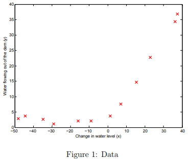
Visualizing the dataset
We will begin by visualizing the dataset containing historical records on the change in the water level, x, and the amount of water flowing out of the dam, y.
This dataset is divided into three parts:
A training set that your model will learn on: X, y
A cross validation set for determining the regularization parameter: Xval, yval
A test set for evaluating performance. These are “unseen” examples which your model did not see during training: Xtest, ytest
The next step of ex5.m will plot the training data (Figure 1). In the following parts, you will implement linear regression and use that to fit a straight line to the data and plot learning curves.
Following that, you will implement polynomial regression to find a better fit to the data.
Regularized linear regression cost function
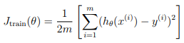
Recall that regularized linear regression has the following cost function:
where λ is a regularization parameter which controls the degree of regularization (thus, help preventing overfitting).
The regularization term puts a penalty on the overal cost J.
As the magnitudes of the model parameters \( \theta_j \) increase, the penalty increases as well.
Note that you should not regularize the \( \theta_0 \) term.
(In Octave/MATLAB, the \( \theta_0 \) term is represented as theta(1) since indexing in Octave/MATLAB starts from 1).
You should now complete the code in the file linearRegCostFunction.m. Your task is to write a function to calculate the regularized linear regression cost function.
If possible, try to vectorize your code and avoid writing loops.
When you are finished, the next part of ex5.m will run your cost function using theta initialized at [1; 1].
You should expect to see an output of 303.993.
Tutorial : ex5 tutorial linearRegCostFunction
The first line of code will compute a vector 'h' containing all of the hypothesis values - one for each training example (i.e. for each row of X).
The hypothesis (also called the prediction) is simply the product of X and theta. So your first line of code is.
h = {multiply X and theta, in the proper order that the inner dimensions match}Since X is size (m x n) and theta is size (n x 1), you arrange the order of operators so the result is size (m x 1).
The second line of code will compute the difference between the hypothesis and y - that's the error for each training example. Difference means subtract.
error = {the difference between h and y}The third line of code will compute the square of each of those error terms (using element-wise exponentiation),
An example of using element-wise exponentiation - try this in your workspace command line so you see how it works.
v = [-2 3]
v_sqr = v.^2
So, now you should compute the squares of the error terms:
error_sqr = {use what you have learned}Next, here's an example of how the sum function works (try this from your command line)
q = sum([1 2 3])
Now, we'll finish the last two steps all in one line of code. You need to compute the sum of the error_sqr vector, and scale the result (multiply) by 1/(2*m). That completed sum is the cost value J.
J = {multiply 1/(2*m) times the sum of the error_sqr vector}So now you've got unregularized cost J
For the cost regularization:
Set theta(1) to 0.
Compute the sum of all of the theta values squared. One handy way to do this is sum(theta.^2). Since theta(1) has been forced to zero, it doesn't add to the regularization term.
Now scale this value by lambda / (2*m), and add it to the unregularized cost.
Regularized linear regression gradient
Correspondingly, the partial derivative of regularized linear regression’s cost for \( \theta_j \) is defined as
In linearRegCostFunction.m, add code to calculate the gradient, returning it in the variable grad.
When you are finished, the next part of ex5.m will run your gradient function using theta initialized at [1; 1]. You should expect to see a gradient of [-15.30; 598.250].
ex5 tutorial linearRegCostFunction
The hypothesis is a vector, formed by multiplying the X matrix and the theta vector. X has size (m x n), and theta is (n x 1), so the product is (m x 1). That's good, because it's the same size as 'y'. Call this hypothesis vector 'h'.
The "errors vector" is the difference between the 'h' vector and the 'y' vector.
The change in theta (the "gradient") is the sum of the product of X and the "errors vector", scaled by 1/m. Since X is (m x n), and the error vector is (m x 1), and the result you want is the same size as theta (which is (n x 1), you need to transpose X before you can multiply it by the error vector.
The vector multiplication automatically includes calculating the sum of the products.
When you're scaling by 1/m, be sure you use enough sets of parenthesis to get the factors correct.
For the gradient regularization:
The regularized gradient term is theta scaled by (lambda / m). Again, since theta(1) has been set to zero, it does not contribute to the regularization term.
Add this vector to the unregularized portion.
ex5 test case linearRegCostFunction
X = [[1 1 1]' magic(3)];
y = [7 6 5]';
theta = [0.1 0.2 0.3 0.4]';
[J g] = linearRegCostFunction(X, y, theta, ?)

%--- results based on value entered for ? (lambda)
--------------------------
lambda = 0  |   lambda = 7
--------------------------
J = 1.3533  |   J = 1.6917
g =         |   g =
   -1.4000  |      -1.4000
   -8.7333  |      -8.2667
   -4.3333  |      -3.6333
   -7.9333  |      -7.0000


X = [1 2 3 4];
y = 5;
theta = [0.1 0.2 0.3 0.4]';
[J g] = linearRegCostFunction(X, y, theta, 7)

% results
J =  3.0150
g =
  -2.0000
  -2.6000
  -3.9000
  -5.2000
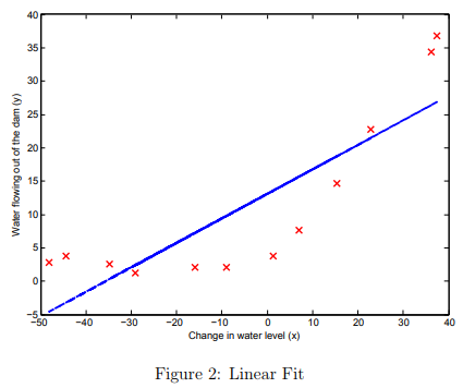
Fitting linear regression
Once your cost function and gradient are working correctly, the next part of ex5.m will run the code in trainLinearReg.m to compute the optimal values of θ. This training function uses fmincg to optimize the cost function.
In this part, we set regularization parameter \( \lambda \) to zero. Because our current implementation of linear regression is trying to fit a 2-dimensional θ, regularization will not be incredibly helpful for a \( \theta \) of such low dimension.
In the later parts of the exercise, you will be using polynomial regression with regularization.
Finally, the ex5.m script should also plot the best fit line, resulting in an image similar to Figure 2.
The best fit line tells us that the model is not a good fit to the data because the data has a non-linear pattern.
While visualizing the best fit as shown is one possible way to debug your learning algorithm, it is not always easy to visualize the data and model.
In the next section, you will implement a function to generate learning curves that can help you debug your learning algorithm even if it is not easy to visualize the data.
Bias-variance
An important concept in machine learning is the bias-variance tradeoff.
Models with high bias are not complex enough for the data and tend to underfit, while models with high variance overfit to the training data.
In this part of the exercise, you will plot training and test errors on a learning curve to diagnose bias-variance problems
Learning curves
You will now implement code to generate the learning curves that will be useful in debugging learning algorithms.
Recall that a learning curve plots training and cross validation error as a function of training set size. Your job is to fill in learningCurve.m so that it returns a vector of errors for the training set and cross validation set.
To plot the learning curve, we need a training and cross validation set error for different training set sizes.
To obtain different training set sizes, you should use different subsets of the original training set X. Specifically, for a training set size of i, you should use the first i examples (i.e., X(1:i,:) and y(1:i)).
You can use the trainLinearReg function to find the θ parameters. Note that the lambda is passed as a parameter to the learningCurve function.
After learning the \( \theta \) parameters, you should compute the error on the training and cross validation sets.
Recall that the training error for a dataset is defined as
In particular, note that the training error does not include the regularization term.
One way to compute the training error is to use your existing cost function and set \( \lambda \) to 0 only when using it to compute the training error and cross validation error.
When you are computing the training set error, make sure you compute it on the training subset (i.e., X(1:n,:) and y(1:n)) (instead of the entire training set).
However, for the cross validation error, you should compute it over the entire cross validation set. You should store the computed errors in the vectors error train and error val.
When you are finished, ex5.m wil print the learning curves and produce a plot similar to Figure 3.
In Figure 3, you can observe that both the train error and cross validation error are high when the number of training examples is increased.
This reflects a high bias problem in the model – the linear regression model is
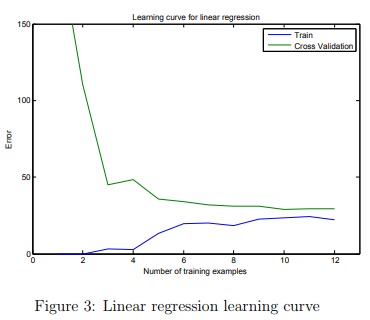
too simple and is unable to fit our dataset well. In the next section, you will implement polynomial regression to fit a better model for this dataset.
ex5: tips for learningCurve()
Step 1) Use a for-loop to iterate over the length of the training set. The "Hint" in learningCurve.m gives you the code to use.
Step 2) Create a subset of the "X" matrix and the 'y' vector, using the elements 1 through 'i'. The first "Note" in learningCurve.m gives you the code to use. This causes the training set size to increase by one for each iteration through the training set. You will use this subset for training (Step 3) and measuring the training set error (Step 4).
Step 3) Use the trainLinearReg() function to learn the theta vector for the current size of training set (see page 6 of ex5.pdf).
Step 4) Then use your cost function to compute the training set error. Do not include regularization. Store the training set cost in error_train(i).
Step 5) Then use your cost function to compute the validation set error, using Xval and yval. Do not include regularization. Do not create any subsets of the validation set. Store the validation set error in error_val(i).
Tips:
Use the lambda parameter - from the learningCurve() parameter list - every time you call trainLinearReg().
do not set lambda = 0 inside the learningCurve() function. You are going to experiment with different lambda values in ex5.m, and the submit grader doesn't use lambda = 0. So do not hard-code lambda = 0 inside the learningCurve() function.
When you compute the training set error and the validation set error, use your cost function with a zero for the lambda parameter. We want to measure the error in the hypothesis, without including any additional penalties for the theta values.
When you run the "ex5" script, you may get some "divide by zero" warnings. These are expected and normal. fmincg() generates "divide by zero" warnings whenever the training set has only one or two examples. Do not worry about it.
Test case for learningCurve()
X = [ones(5,1) reshape(-5:4,5,2)];
y = [-2:2]';
Xval=[X;X]/10;
yval=[y;y]/10;
[et ev] = learningCurve(X,y,Xval,yval,1)

You should get these results:

et =

   0.000000
   0.031250
   0.013333
   0.005165
   0.002268

ev =

  3.0000e-002
  5.3125e-003
  6.0000e-004
  9.2975e-005
  2.2676e-005

Here are the theta values for each size of training set:

% m = 1
theta =
  -2.00000
   0.00000
   0.00000

% m = 2
theta =
  -0.50000
   0.25000
   0.25000

% m = 3
theta =
   0.20000
   0.40000
   0.40000

% m = 4
theta =
   0.40909
   0.45455
   0.45455

% m = 5
theta =
   0.47619
   0.47619
   0.47619
Polynomial regression
The problem with our linear model was that it was too simple for the data and resulted in underfitting (high bias). In this part of the exercise, you will address this problem by adding more features.
For use polynomial regression, our hypothesis has the form:
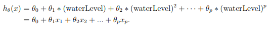
Notice that by defining x1 = (waterLevel), x2 = (waterLevel)2 , . . . , xp = (waterLevel)p , we obtain a linear regression model where the features are the various powers of the original value (waterLevel).
Now, you will add more features using the higher powers of the existing feature x in the dataset. Your task in this part is to complete the code in polyFeatures.m so that the function maps the original training set X of size m × 1 into its higher powers.
Specifically, when a training set X of size m × 1 is passed into the function, the function should return a m×p matrix X_poly, where column 1 holds the original values of X, column 2 holds the values of X.^2, column 3 holds the values of X.^3, and so on.
Note that you don’t have to account for the zero-eth power in this function.
Now you have a function that will map features to a higher dimension, and Part 6 of ex5.m will apply it to the training set, the test set, and the cross validation set (which you haven’t used yet).
Tutorial for polyFeatures()
There are a couple of different methods that work for the polyFeatures() function.
One is to use the bsxfun() function, with the @power operator, like this:
X_poly = bsxfun(@power, vector1, vector2)
where vector1 is a column vector of the feature values 'X', and vector2 is a row vector of exponents from 1 to 'p'.
Other options involve using the element-wise exponent operator '.^', and converting both X and the vector of exponent values into equal-sized matrices by multiplying each by a vectors of all-ones.
Test Case for polyFeatures()
polyFeatures([1:3]',4)

ans =
    1    1    1    1
    2    4    8   16
    3    9   27   81

polyFeatures([1:7]',4)

ans =

      1      1      1      1
      2      4      8     16
      3      9     27     81
      4     16     64    256
      5     25    125    625
      6     36    216   1296
      7     49    343   2401
Learning Polynomial Regression
After you have completed polyFeatures.m, the ex5.m script will proceed to train polynomial regression using your linear regression cost function.
Keep in mind that even though we have polynomial terms in our feature vector, we are still solving a linear regression optimization problem.
The polynomial terms have simply turned into features that we can use for linear regression. We are using the same cost function and gradient that you wrote for the earlier part of this exercise.
For this part of the exercise, you will be using a polynomial of degree 8. It turns out that if we run the training directly on the projected data, will not work well as the features would be badly scaled (e.g., an example with x = 40 will now have a feature \( x_8 = 40^8 = 6.5 × 10^{12} \). Therefore, you will need to use feature normalization.
Before learning the parameters \( \theta \) for the polynomial regression, ex5.m will first call featureNormalize and normalize the features of the training set, storing the mu, sigma parameters separately.
We have already implemented this function for you and it is the same function from the first exercise.
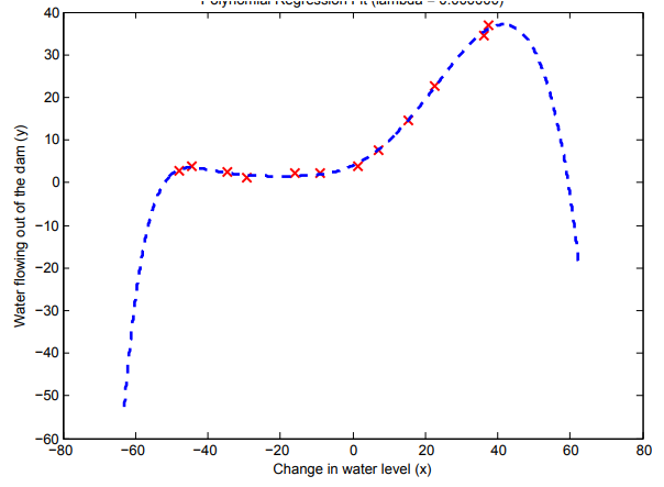
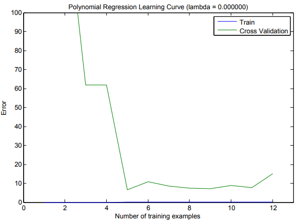
After learning the parameters \( \theta \), you should see two plots (Figure 4,5) generated for polynomial regression with \( \lambda \) = 0.
From Figure 4, you should see that the polynomial fit is able to follow the datapoints very well - thus, obtaining a low training error.
However, the polynomial fit is very complex and even drops off at the extremes.
This is an indicator that the polynomial regression model is overfitting the training data and will not generalize well.
To better understand the problems with the unregularized (\( \lambda \) = 0) model, you can see that the learning curve (Figure 5) shows the same effect where the low training error is low, but the cross validation error is high.
There is a gap between the training and cross validation errors, indicating a high variance problem.
One way to combat the overfitting (high-variance) problem is to add regularization to the model. In the next section, you will get to try different \( \lambda \) parameters to see how regularization can lead to a better model
Selecting λ using a cross validation set
From the previous parts of the exercise, you observed that the value of λ can significantly affect the results of regularized polynomial regression on the training and cross validation set.
In particular, a model without regularization (λ = 0) fits the training set well, but does not generalize. Conversely, a model with too much regularization (λ = 100) does not fit the training set and testing set well.
A good choice of λ (e.g., λ = 1) can provide a good fit to the data.
In this section, you will implement an automated method to select the λ parameter.
Concretely, you will use a cross validation set to evaluate how good each λ value is.
After selecting the best λ value using the cross validation set, we can then evaluate the model on the test set to estimate how well the model will perform on actual unseen data.
Your task is to complete the code in validationCurve.m. Specifically, you should should use the trainLinearReg function to train the model using different values of λ and compute the training error and cross validation error.
You should try λ in the following range: {0, 0.001, 0.003, 0.01, 0.03, 0.1, 0.3, 1, 3, 10}.
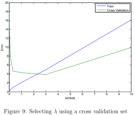
After you have completed the code, the next part of ex5.m will run your function can plot a cross validation curve of error v.s. λ that allows you select which λ parameter to use. You should see a plot similar to Figure 9.
In this figure, we can see that the best value of λ is around 3. Due to randomness in the training and validation splits of the dataset, the cross validation error can sometimes be lower than the training error.
Tutorial : Validation curve
Train using the whole training set and a value for lambda
Measure Jtrain and Jcv using the entire training and validation sets, with lambda set to 0
For validationCurve(), you always use the entire training set, and the entire validation set. The only item you are varying is the value of lambda when you compute theta on the training set.
Also, do not use regularization when measuring the training error and the validation error.
Test Case for validationCurve()
X = [1 2 ; 1 3 ; 1 4 ; 1 5];
y = [7 6 5 4]';
Xval = [1 7 ; 1 -2];
yval = [2 12]';
[lambda_vec, error_train, error_val] = validationCurve(X,y,Xval,yval )

% results:
lambda_vec =
    0.00000
    0.00100
    0.00300
    0.01000
    0.03000
    0.10000
    0.30000
    1.00000
    3.00000
   10.00000

error_train =

   0.00000
   0.00000
   0.00000
   0.00000
   0.00002
   0.00024
   0.00200
   0.01736
   0.08789
   0.27778

error_val =

   0.25000
   0.25055
   0.25165
   0.25553
   0.26678
   0.30801
   0.43970
   1.00347
   2.77539
   6.80556