Introductory Video

• The Machine Learning course includes several programming assignments which you’ll need to finish to complete the course. The assignments require the Octave scientific computing language.




• Octave is a free, open-source application available for many platforms. It has a text interface and an experimental graphical one. Octave is distributed under the GNU Public License, which means that it is always free to download and distribute.




• Use Download to install Octave for windows. "Warning: Do not install Octave 4.0.0";




• Installing Octave on GNU/Linux : On Ubuntu, you can use: sudo apt-get update && sudo apt-get install octave. On Fedora, you can use: sudo yum install octave-forge

• In this exercise, you will implement K-means Clustering and Principal Component Analysis.




• Files included in this exercise can be downloaded here ⇒ : Download




• In this exercise, you will implement the K-means clustering algorithm and apply it to compress an image. In the second part, you will use principal component analysis to find a low-dimensional representation of face images.




• Before starting on the programming exercise, we strongly recommend watching the video lectures and completing the review questions for the associated topics.




• To get started with the exercise, you will need to download the starter code and unzip its contents to the directory where you wish to complete the exercise. If needed, use the cd command in Octave/MATLAB to change to this directory before starting this exercise.




• You can also find instructions for installing Octave/MATLAB in the “Environment Setup Instructions” of the course website.




• Files included in this exercise




• ex7.m - Octave/MATLAB script for the first exercise on K-means
  ex7 pca.m - Octave/MATLAB script for the second exercise on PCA
  ex7data1.mat - Example Dataset for PCA
  ex7data2.mat - Example Dataset for K-means
  ex7faces.mat - Faces Dataset
  bird small.png - Example Image
  displayData.m - Displays 2D data stored in a matrix
  drawLine.m - Draws a line over an exsiting figure
  plotDataPoints.m - Initialization for K-means centroids
  plotProgresskMeans.m - Plots each step of K-means as it proceeds
  runkMeans.m - Runs the K-means algorithm
  submit.m - Submission script that sends your solutions to our servers
  [*] pca.m - Perform principal component analysis
  [*] projectData.m - Projects a data set into a lower dimensional space
  [*] recoverData.m - Recovers the original data from the projection
  [*] findClosestCentroids.m - Find closest centroids (used in K-means)
  [*] computeCentroids.m - Compute centroid means (used in K-means)
  [*] kMeansInitCentroids.m - Initialization for K-means centroids
  * - indicates files you will need to complete
  




• Throughout the first part of the exercise, you will be using the script ex7.m, for the second part you will use ex7_pca.m.




• These scripts set up the dataset for the problems and make calls to functions that you will write.




• You are only required to modify functions in other files, by following the instructions in this assignment.

• In this this exercise, you will implement the K-means algorithm and use it for image compression.




• You will first start on an example 2D dataset that will help you gain an intuition of how the K-means algorithm works.




• After that, you wil use the K-means algorithm for image compression by reducing the number of colors that occur in an image to only those that are most common in that image.




• You will be using ex7.m for this part of the exercise.

• The K-means algorithm is a method to automatically cluster similar data examples together. Concretely, you are given a training set {x⁽¹⁾, ..., x^(m)} (where x⁽ⁱ⁾ ∈ Rⁿ), and want to group the data into a few cohesive “clusters”.




• The intuition behind K-means is an iterative procedure that starts by guessing the initial centroids, and then refines this guess by repeatedly assigning examples to their closest centroids and then recomputing the centroids based on the assignments.




• The K-means algorithm is as follows:




• % Initialize centroids
  centroids = kMeansInitCentroids(X, K);
  for iter = 1:iterations
  % Cluster assignment step: Assign each data point to the
  % closest centroid. idx(i) corresponds to cˆ(i), the index
  % of the centroid assigned to example i
  idx = findClosestCentroids(X, centroids);
  % Move centroid step: Compute means based on centroid
  % assignments
  centroids = computeMeans(X, idx, K);
  end
  




• The inner-loop of the algorithm repeatedly carries out two steps: (i) Assigning each training example x⁽ⁱ⁾ to its closest centroid, and (ii) Recomputing the mean of each centroid using the points assigned to it.




• The K-means algorithm will always converge to some final set of means for the centroids. Note that the converged solution may not always be ideal and depends on the initial setting of the centroids.




• Therefore, in practice the K-means algorithm is usually run a few times with different random initializations.




• One way to choose between these different solutions from different random initializations is to choose the one with the lowest cost function value (distortion).




• You will implement the two phases of the K-means algorithm separately in the next sections.

• In the “cluster assignment” phase of the K-means algorithm, the algorithm assigns every training example x⁽ⁱ⁾ to its closest centroid, given the current positions of centroids.




• Specifically, for every example i we set c⁽ⁱ⁾:= j that minimizes ||x⁽ⁱ⁾ − µ_j||² , where c⁽ⁱ⁾ is the index of the centroid that is closest to x⁽ⁱ⁾ , and µ_j is the position (value) of the j'th centroid.




• Note that c⁽ⁱ⁾ corresponds to idx(i) in the starter code.




• Your task is to complete the code in findClosestCentroids.m.




• This function takes the data matrix X and the locations of all centroids inside centroids and should output a one-dimensional array idx that holds the index (a value in {1, ..., K}, where K is total number of centroids) of the closest centroid to every training example.




• You can implement this using a loop over every training example and every centroid.




• Once you have completed the code in findClosestCentroids.m, the script ex7.m will run your code and you should see the output [1 3 2] corresponding to the centroid assignments for the first 3 examples.

• This tutorial gives a method for findClosestCentroids() by iterating through the centroids. This runs considerably faster than looping through the training examples.




• Create a "distance" matrix of size (m x K) and initialize it to all zeros. 'm' is the number of training examples, K is the number of centroids.




• Use a for-loop over the 1:K centroids.




• Inside this loop, create a column vector of the distance from each training example to that centroid, and store it as a column of the distance matrix. One method is to use the bsxfun) function and the sum() function to calculate the sum of the squares of the differences between each row in the X matrix and a centroid.




• When the for-loop ends, you'll have a matrix of centroid distances.




• Then return idx as the vector of the indexes of the locations with the minimum distance. The result is a vector of size (m x 1) with the indexes of the closest centroids.




• Additional implementation tips on how to use bsxfun():




• bsxfun() means "broadcast function". It applies whatever function you specify (such as @minus) between the 1st argument (a matrix) and the second argument (typically a row vector).




• Here's an example you can enter in your console:




• Q = magic(3)
  D = bsxfun(@minus, Q, [1 2 3])
  




• It returns a value that is the same size as the first argument.




• As implemented for this function, each row in the matrix returned by bsxfun() is the differences between that row of X and each of the features of one of the centroids.




• Then, for each row, you compute the sum of the squares of those differences. Here is code that does it.




• sum(D.^2,2)
  




• Note that if you leave off the ',2' part, then sum() will sum over the rows, and you'll instead get a (1xn) vector. Using ',2' tells sum() to work over the columns, so you'll get a (m x 1) result.




• We repeat this process for each of the centroids. Once we have the squared distance between each example and each centroid, we then return the index where the min() value was found for each example.

• % ========== findClosestCentroids() ============
  X = reshape(sin(1:50), 10, 5);
  cent = X(7:10,:);
  idx = findClosestCentroids(X, cent)
  
  % result
  idx =
     1
     2
     3
     4
     4
     1
     1
     2
     3
     4
  
  % additional information
  % these are the "distances" for each example, computed as the sum
  % of the squares of the differences for each feature.
  debug> dist
  dist =
  
      0.18685    1.26617    6.26061   10.23971
      3.68554    0.21768    1.31858    5.63745
      9.03781    3.83809    0.19602    1.12150
     10.66224    8.13823    3.26444    0.18322
      6.96941    9.06864    7.60682    3.58933
      2.09490    6.51432    9.97120    8.94869
      0.00000    2.30339    7.66348   10.81361
      2.30339    0.00000    2.49799    7.16213
      7.66348    2.49799    0.00000    2.12753
     10.81361    7.16213    2.12753    0.00000
  

• Given assignments of every point to a centroid, the second phase of the algorithm recomputes, for each centroid, the mean of the points that were assigned to it. Specifically, for every centroid k we set \( \mu_k := \frac{1}{|C_k|} \sum_{i \in C_k} x^{(i)} \)




• where Ck is the set of examples that are assigned to centroid k. Concretely, if two examples say x⁽³⁾ and x⁽⁵⁾ are assigned to centroid k = 2, then you should update \( \mu_2 = \frac{1}{2} (x^{(3)} + x^{(5)}) \)




• You should now complete the code in computeCentroids.m. You can implement this function using a loop over the centroids. You can also use a loop over the examples; but if you can use a vectorized implementation that does not use such a loop, your code may run faster.




• Once you have completed the code in computeCentroids.m, the script ex7.m will run your code and output the centroids after the first step of Kmeans.

• The method in this tutorial iterates over the centroids.




• The function computeCentroids is called with parameters "X, "idx" and "K".




• "K" is the number of centroids.




• "idx" is a vector with one entry for each example in "X", which tells you which centroid each example is assigned to. The values range from 1 to K, so you will need a for-loop over that range.




• You can get a selection of all of the indexes for each centroid with: sel = find(idx == i) % where i ranges from 1 to K




• Now we want to compute the mean of all these selected examples, and assign it as the new centroid value: centroids(i,:) = mean(X(sel,:))




• (Note that this method breaks if sel is a null vector (i.e. if no examples are assigned to centroid 'i'. In that case, probably should only update centroid(i,:) if sel is a non-null vector.




• Repeat this procedure all each centroid. The function returns the computed centroid values.

• % ========== computeCentroids() ============
  X = reshape([1:24],8,3);
  computeCentroids(X, [1 1 3 3 4 4 2 2]',4)
  
  % result
  ans =
      1.5000    9.5000   17.5000
      7.5000   15.5000   23.5000
      3.5000   11.5000   19.5000
      5.5000   13.5000   21.5000
  

• 




• After you have completed the two functions (findClosestCentroids and computeCentroids), the next step in ex7.m will run the K-means algorithm on a toy 2D dataset to help you understand how K-means works.




• Your functions are called from inside the runKmeans.m script. We encourage you to take a look at the function to understand how it works.




• Notice that the code calls the two functions you implemented in a loop.




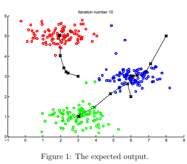
• When you run the next step, the K-means code will produce a visualization that steps you through the progress of the algorithm at each iteration.




• Press enter multiple times to see how each step of the K-means algorithm changes the centroids and cluster assignments. At the end, your figure should look as the one displayed in Figure 1.

• The initial assignments of centroids for the example dataset in ex7.m were designed so that you will see the same figure as in Figure 1.




• In practice, a good strategy for initializing the centroids is to select random examples from the training set.




• In this part of the exercise, you should complete the function kMeansInitCentroids.m with the following code:




• % Initialize the centroids to be random examples
  % Randomly reorder the indices of examples
  randidx = randperm(size(X, 1));
  % Take the first K examples as centroids
  centroids = X(randidx(1:K), :);
  




• The code above first randomly permutes the indices of the examples (using randperm). Then, it selects the first K examples based on the random permutation of the indices. This allows the examples to be selected at random without the risk of selecting the same example twice.

• 




• In this exercise, you will apply K-means to image compression.




• In a straightforward 24-bit color representation of an image,2 each pixel is represented as three 8-bit unsigned integers (ranging from 0 to 255) that specify the red, green and blue intensity values.




• This encoding is often refered to as the RGB encoding. Our image contains thousands of colors, and in this part of the exercise, you will reduce the number of colors to 16 colors.




• By making this reduction, it is possible to represent (compress) the photo in an efficient way.




• Specifically, you only need to store the RGB values of the 16 selected colors, and for each pixel in the image you now need to only store the index of the color at that location (where only 4 bits are necessary to represent 16 possibilities).




• In this exercise, you will use the K-means algorithm to select the 16 colors that will be used to represent the compressed image. Concretely, you will treat every pixel in the original image as a data example and use the K-means algorithm to find the 16 colors that best group (cluster) the pixels in the 3- dimensional RGB space.




• Once you have computed the cluster centroids on the image, you will then use the 16 colors to replace the pixels in the original image.

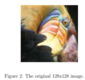
• In Octave/MATLAB, images can be read in as follows:




• % Load 128x128 color image (bird small.png)
  A = imread('bird small.png');
  % You will need to have installed the image package to used
  % imread. If you do not have the image package installed, you
  % should instead change the following line to
  %
  % load('bird small.mat'); % Loads the image into the variable A
  




• This creates a three-dimensional matrix A whose first two indices identify a pixel position and whose last index represents red, green, or blue. For example, A(50, 33, 3) gives the blue intensity of the pixel at row 50 and column 33.




• The code inside ex7.m first loads the image, and then reshapes it to create an m × 3 matrix of pixel colors (where m = 16384 = 128 × 128), and calls your K-means function on it.




• After finding the top K = 16 colors to represent the image, you can now assign each pixel position to its closest centroid using the findClosestCentroids function.




• This allows you to represent the original image using the centroid assignments of each pixel. Notice that you have significantly reduced the number of bits that are required to describe the image.




• The original image required 24 bits for each one of the 128×128 pixel locations, resulting in total size of 128 × 128 × 24 = 393, 216 bits. The new representation requires some overhead storage in form of a dictionary of 16 colors, each of which require 24 bits, but the image itself then only requires 4 bits per pixel location.




• The final number of bits used is therefore 16 × 24 + 128 × 128 × 4 = 65, 920 bits, which corresponds to compressing the original image by about a factor of 6.




• 




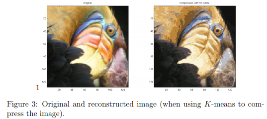
• Finally, you can view the effects of the compression by reconstructing the image based only on the centroid assignments. Specifically, you can replace each pixel location with the mean of the centroid assigned to it. Figure 3 shows the reconstruction we obtained. Even though the resulting image retains most of the characteristics of the original, we also see some compression artifacts.