Setting Up Your Programming Assignment Environment
Introductory Video
The Machine Learning course includes several programming assignments which you’ll need to finish to complete the course. The assignments require the Octave scientific computing language.
Octave is a free, open-source application available for many platforms. It has a text interface and an experimental graphical one. Octave is distributed under the GNU Public License, which means that it is always free to download and distribute.
Use Download to install Octave for windows. "Warning: Do not install Octave 4.0.0";
Installing Octave on GNU/Linux : On Ubuntu, you can use: sudo apt-get update && sudo apt-get install octave. On Fedora, you can use: sudo yum install octave-forge
Introduction - Principal Component Analysis
In this exercise, you will implement Principal Component Analysis.
Files included in this exercise can be downloaded here ⇒ : Download
In this exercise, you will use principal component analysis (PCA) to perform dimensionality reduction.
You will first experiment with an example 2D dataset to get intuition on how PCA works, and then use it on a bigger dataset of 5000 face image dataset.
The provided script, ex7_pca.m, will help you step through the first half of the exercise.
Example Dataset
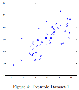
To help you understand how PCA works, you will first start with a 2D dataset which has one direction of large variation and one of smaller variation.
The script ex7_pca.m will plot the training data (Figure 4). In this part of the exercise, you will visualize what happens when you use PCA to reduce the data from 2D to 1D.
In practice, you might want to reduce data from 256 to 50 dimensions, say; but using lower dimensional data in this example allows us to visualize the algorithms better.
Step 1: Implementing PCA
In this part of the exercise, you will implement PCA. PCA consists of two computational steps: First, you compute the covariance matrix of the data.
Then, you use Octave/MATLAB’s SVD function to compute the eigenvectors \( U_1, U_2, . . . , U_n \). These will correspond to the principal components of variation in the data.
Before using PCA, it is important to first normalize the data by subtracting the mean value of each feature from the dataset, and scaling each dimension so that they are in the same range.
In the provided script ex7_pca.m, this normalization has been performed for you using the featureNormalize function.
After normalizing the data, you can run PCA to compute the principal components.
You task is to complete the code in pca.m to compute the principal components of the dataset.
First, you should compute the covariance matrix of the data, which is given by: \( \sigma = \frac{1}{m} X^TX \)
where X is the data matrix with examples in rows, and m is the number of examples.
Note that Σ is a n × n matrix and not the summation operator. After computing the covariance matrix, you can run SVD on it to compute the principal components.
In Octave/MATLAB, you can run SVD with the following command: [U, S, V] = svd(Sigma), where U will contain the principal components and S will contain a diagonal matrix.
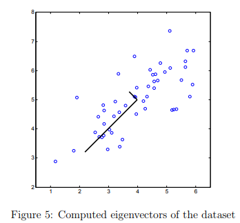
Once you have completed pca.m, the ex7_pca.m script will run PCA on the example dataset and plot the corresponding principal components found (Figure 5).
The script will also output the top principal component (eigenvector) found, and you should expect to see an output of about [-0.707 -0.707].
(It is possible that Octave/MATLAB may instead output the negative of this, since U1 and −U1 are equally valid choices for the first principal component.)
Tutorials for ex7_pca : pca()
Compute the transpose of X times X, scale by 1/m, and use the svd() function to return the U, S, and V matrices.
X is size (m x n), so "X transpose X" and U are both size (n x n)
(note: the feature matrix X has already been normalized, see ex7_pca.m)
Testcases for ex7_pca : pca()
% ========== pca() ============
[U, S] = pca(sin([0 1; 2 3; 4 5]))

% result
U =
  -0.65435  -0.75619
  -0.75619   0.65435

S =
Diagonal Matrix
   0.79551  0
   0        0.22019
Dimensionality Reduction with PCA
After computing the principal components, you can use them to reduce the feature dimension of your dataset by projecting each example onto a lower dimensional space, x(i) → z(i) (e.g., projecting the data from 2D to 1D).
In this part of the exercise, you will use the eigenvectors returned by PCA and project the example dataset into a 1-dimensional space.
In practice, if you were using a learning algorithm such as linear regression or perhaps neural networks, you could now use the projected data instead of the original data.
By using the projected data, you can train your model faster as there are less dimensions in the input.
Step 2: Projecting the data onto the principal components
You should now complete the code in projectData.m. Specifically, you are given a dataset X, the principal components U, and the desired number of dimensions to reduce to K.
You should project each example in X onto the top K components in U.
Note that the top K components in U are given by the first K columns of U, that is Ureduce = U(:, 1:K).
Once you have completed the code in projectData.m, ex7 pca.m will project the first example onto the first dimension and you should see a value of about 1.481 (or possibly -1.481, if you got −U1 instead of U1).
Tutorials for ex7_pca : projectData()
In projectData.m, make the following change in the Instructions section:
% projection_k = x' * U(:, 1:k);
Return Z, the product of X and the first 'K' columns of U.
X is size (m x n), and the portion of U is (n x K). Z is size (m x K).
Testcases for ex7_pca : projectData()
% ========== projectData() ============
X = sin(reshape([0:11],4,3));
projectData(X, magic(3), 2)

% result
ans =
   1.68703   5.12021
   5.50347  -0.24408
   4.26005  -5.38397
  -0.90004  -5.57386
Step 3: Reconstructing an approximation of the data
After projecting the data onto the lower dimensional space, you can approximately recover the data by projecting them back onto the original high dimensional space.
Your task is to complete recoverData.m to project each example in Z back onto the original space and return the recovered approximation in X_rec.
Once you have completed the code in recoverData.m, ex7_pca.m will recover an approximation of the first example and you should see a value of about [-1.047 -1.047].
Tutorials for ex7_pca : recoverData()
Return X_rec, the product of Z and the first 'K' columns of U.
Dimensional analysis:
The original data set was size (m x n)
Z is size (m x K), where 'K' is the number of features we retained.
U is size (n x n), where 'n' is the number of features in the original set.
So "U(:,1:K)" is size (n x K).
So to restore an approximation of the original data set using only K features, we multiply (m x K) * (K x n), giving a (m x n) result.
Testcases for ex7_pca : recoverData()
% ========== recoverData() ============
Q = reshape([1:15],5,3);
recoverData(Q, magic(5), 3)

% result
ans =
   172   130   183   291   394
   214   165   206   332   448
   256   200   229   373   502
   298   235   252   414   556
   340   270   275   455   610
Visualizing the projections
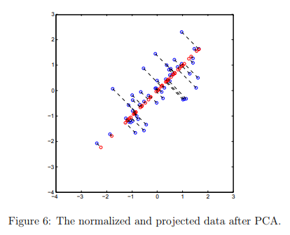
After completing both projectData and recoverData, ex7 pca.m will now perform both the projection and approximate reconstruction to show how the projection affects the data.
In Figure 6, the original data points are indicated with the blue circles, while the projected data points are indicated with the red circles.
The projection effectively only retains the information in the direction given by U1
Face Image Dataset
In this part of the exercise, you will run PCA on face images to see how it can be used in practice for dimension reduction.
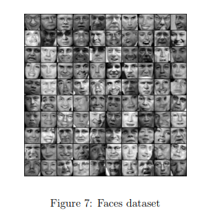
The dataset ex7faces.mat contains a dataset X of face images, each 32 × 32 in grayscale.
Each row of X corresponds to one face image (a row vector of length 1024).
The next step in ex7_pca.m will load and visualize the first 100 of these face images (Figure 7).
PCA on Faces
To run PCA on the face dataset, we first normalize the dataset by subtracting the mean of each feature from the data matrix X.
The script ex7_pca.m will do this for you and then run your PCA code.
After running PCA, you will obtain the principal components of the dataset.
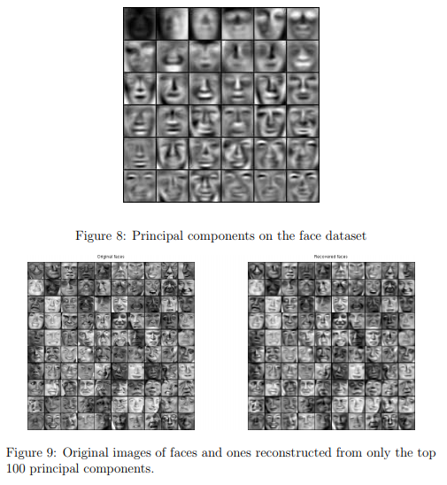
Notice that each principal component in U (each row) is a vector of length n (where for the face dataset, n = 1024).
It turns out that we can visualize these principal components by reshaping each of them into a 32 × 32 matrix that corresponds to the pixels in the original dataset.
The script ex7_pca.m displays the first 36 principal components that describe the largest variations (Figure 8).
If you want, you can also change the code to display more principal components to see how they capture more and more details.
Dimensionality Reduction
Now that you have computed the principal components for the face dataset, you can use it to reduce the dimension of the face dataset.
This allows you to use your learning algorithm with a smaller input size (e.g., 100 dimensions) instead of the original 1024 dimensions.
This can help speed up your learning algorithm.
The next part in ex7_pca.m will project the face dataset onto only the first 100 principal components.
Concretely, each face image is now described by a vector z(i) ∈ R100.
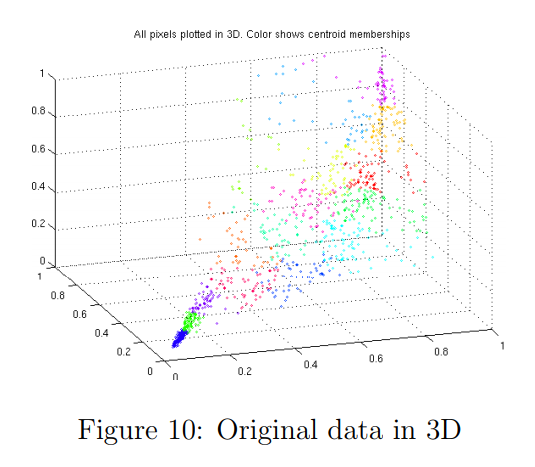
To understand what is lost in the dimension reduction, you can recover the data using only the projected dataset.
In ex7_pca.m, an approximate recovery of the data is performed and the original and projected face images are displayed side by side (Figure 9).
From the reconstruction, you can observe that the general structure and appearance of the face are kept while the fine details are lost.
This is a remarkable reduction (more than 10×) in the dataset size that can help speed up your learning algorithm significantly.
For example, if you were training a neural network to perform person recognition (gven a face image, predict the identitfy of the person), you can use the dimension reduced input of only a 100 dimensions instead of the original pixels.
Optional (ungraded) exercise: PCA for visualization
In the earlier K-means image compression exercise, you used the K-means algorithm in the 3-dimensional RGB space.
In the last part of the ex7_pca.m script, we have provided code to visualize the final pixel assignments in this 3D space using the scatter function.
Each data point is colored according to the cluster it has been assigned to. You can drag your mouse on the figure to rotate and inspect this data in 3 dimensions.
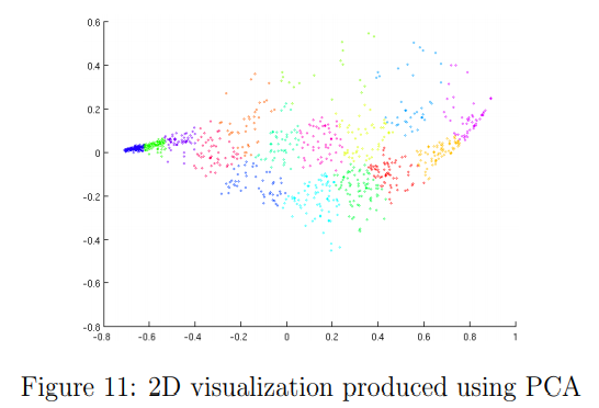
It turns out that visualizing datasets in 3 dimensions or greater can be cumbersome. Therefore, it is often desirable to only display the data in 2D even at the cost of losing some information.
In practice, PCA is often used to reduce the dimensionality of data for visualization purposes.
In the next part of ex7_pca.m, the script will apply your implementation of PCA to the 3- dimensional data to reduce it to 2 dimensions and visualize the result in a 2D scatter plot.
The PCA projection can be thought of as a rotation that selects the view that maximizes the spread of the data, which often corresponds to the “best” view.