Introductory Video

• The Machine Learning course includes several programming assignments which you’ll need to finish to complete the course. The assignments require the Octave scientific computing language.




• Octave is a free, open-source application available for many platforms. It has a text interface and an experimental graphical one. Octave is distributed under the GNU Public License, which means that it is always free to download and distribute.




• Use Download to install Octave for windows. "Warning: Do not install Octave 4.0.0";




• Installing Octave on GNU/Linux : On Ubuntu, you can use: sudo apt-get update && sudo apt-get install octave. On Fedora, you can use: sudo yum install octave-forge

• In this exercise, you will implement Anomaly Detection Systems.




• Files included in this exercise can be downloaded here ⇒ : Download

• In this exercise, you will implement the anomaly detection algorithm and apply it to detect failing servers on a network. In the second part, you will use collaborative filtering to build a recommender system for movies.




• To get started with the exercise, you will need to download the starter code (given above) and unzip its contents to the directory where you wish to complete the exercise.




• If needed, use the cd command in Octave/MATLAB to change to this directory before starting this exercise.




• You can also find instructions for installing Octave/MATLAB above.




• Files included in this exercise




• ex8.m - Octave/MATLAB script for first part of exercise
  ex8_cofi.m - Octave/MATLAB script for second part of exercise
  ex8data1.mat - First example Dataset for anomaly detection
  ex8data2.mat - Second example Dataset for anomaly detection
  ex8_movies.mat - Movie Review Dataset
  ex8_movieParams.mat - Parameters provided for debugging
  multivariateGaussian.m - Computes the probability density function
  for a Gaussian distribution
  visualizeFit.m - 2D plot of a Gaussian distribution and a dataset
  checkCostFunction.m - Gradient checking for collaborative filtering
  computeNumericalGradient.m - Numerically compute gradients
  fmincg.m - Function minimization routine (similar to fminunc)
  loadMovieList.m - Loads the list of movies into a cell-array
  movie ids.txt - List of movies
  normalizeRatings.m - Mean normalization for collaborative filtering
  submit.m - Submission script that sends your solutions to our servers
  [*] estimateGaussian.m - Estimate the parameters of a Gaussian distribution
  with a diagonal covariance matrix
  [*] selectThreshold.m - Find a threshold for anomaly detection
  [*] cofiCostFunc.m - Implement the cost function for collaborative filtering
  




• * indicates files you will need to complete




• Throughout the first part of the exercise (anomaly detection) you will be using the script ex8.m. For the second part of collaborative filtering, you will use ex8 cofi.m.




• These scripts set up the dataset for the problems and make calls to functions that you will write. You are only required to modify functions in other files, by following the instructions in this assignment

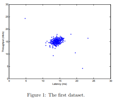
• In this exercise, you will implement an anomaly detection algorithm to detect anomalous behavior in server computers. The features measure the throughput (mb/s) and latency (ms) of response of each server.




• While your servers were operating, you collected m = 307 examples of how they were behaving, and thus have an unlabeled dataset {x⁽¹⁾, . . . , x^(m)}.




• You suspect that the vast majority of these examples are “normal” (non-anomalous) examples of the servers operating normally, but there might also be some examples of servers acting anomalously within this dataset.




• You will use a Gaussian model to detect anomalous examples in your dataset. You will first start on a 2D dataset that will allow you to visualize what the algorithm is doing.




• On that dataset you will fit a Gaussian distribution and then find values that have very low probability and hence can be considered anomalies.




• After that, you will apply the anomaly detection algorithm to a larger dataset with many dimensions. You will be using ex8.m for this part of the exercise.




• The first part of ex8.m will visualize the dataset as shown in Figure 1




• 

• To perform anomaly detection, you will first need to fit a model to the data’s distribution




• Given a training set {x⁽¹⁾, ..., x^(m)} (where x⁽ⁱ⁾ ∈ Rⁿ), you want to estimate the Gaussian distribution for each of the features x_i .




• For each feature i = 1 . . . n, you need to find parameters µ_i and σ²_i that fit the data in the i-th dimension \( {x^{(1)}_i, ..., x^{(m)}_i} \) (the i-th dimension of each example).




• The Gaussian distribution is given by




• \( p(x; \mu, \sigma^2) = \frac{1}{\sqrt{2*\pi*\sigma}} exp(- \frac{(x - \mu)^2}{2\sigma^2}) \)




• where µ is the mean and σ² controls the variance.

• You can estimate the parameters, (µ_i, σ²_i), of the i-th feature by using the following equations.




• To estimate the mean, you will use:




• \( \mu_i = \frac{1}{m} \sum_{j = 1}^{m} x_i^{(j)} \)




• and




• \( \sigma^2 = \frac{1}{m} \sum_{j = 1}^{m} (x^{(i)} - \mu)^2 \)




• Your task is to complete the code in estimateGaussian.m.




• This function takes as input the data matrix X and should output an n-dimension vector mu that holds the mean of all the n features and another n-dimension vector sigma2 that holds the variances of all the features.




• You can implement this using a for-loop over every feature and every training example (though a vectorized implementation might be more efficient; feel free to use a vectorized implementation if you prefer).




• Note that in Octave/MATLAB, the var function will (by default) use \( \frac{1}{m−1} \) , instead of \( \frac{1}{m} \), when computing σ²_i.




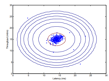
• Once you have completed the code in estimateGaussian.m, the next part of ex8.m will visualize the contours of the fitted Gaussian distribution. You should get a plot similar to Figure 2. From your plot, you can see that most of the examples are in the region with the highest probability, while the anomalous examples are in the regions with lower probabilities.




• 

• Test 1a (Estimate Gaussian Parameters):
  input:
  X = sin(magic(4));
  X = X(:,1:3);
  [mu sigma2] = estimateGaussian(X)
  output:
  mu =
    -0.3978779  0.3892253  -0.0080072
  sigma2 =
     0.27795    0.65844   0.20414
  

• Now that you have estimated the Gaussian parameters, you can investigate which examples have a very high probability given this distribution and which examples have a very low probability.




• The low probability examples are more likely to be the anomalies in our dataset. One way to determine which examples are anomalies is to select a threshold based on a cross validation set.




• In this part of the exercise, you will implement an algorithm to select the threshold ε using the F1 score on a cross validation set.




• You should now complete the code in selectThreshold.m. For this, we will use a cross validation set \( {(x^{(1)}_{cv} , y^{(1)}_{cv} } ) \) , . . . , \( (x^{(mcv)}_{cv} , y^{(mcv)}_{(cv)}) \), where the label y = 1 corresponds to an anomalous example, and y = 0 corresponds to a normal example.




• For each cross validation example, we will compute p(x(i)cv).




• The vector of all of these probabilities \( p(x^{(1)}_{cv}), . . . , p(x^{(mcv)}_{cv}) \) is passed to selectThreshold.m in the vector pval. The corresponding labels \( y^{(1)}_{cv} , . . . , y^{(mcv)}_{cv} \) is passed to the same function in the vector yval




• The function selectThreshold.m should return two values; the first is the selected threshold ε. If an example x has a low probability p(x) < ε, then it is considered to be an anomaly.




• The function should also return the F1 score, which tells you how well you’re doing on finding the ground truth anomalies given a certain threshold.




• For many different values of ε, you will compute the resulting F1 score by computing how many examples the current threshold classifies correctly and incorrectly.




• The F1 score is computed using precision (prec) and recall (rec):




• \( F_1 = \frac{2 · prec · rec}{prec + rec} \)




• You compute precision and recall by:




• \( prec = \frac{tp}{tp + fp} \)




• \( rec = \frac{tp}{tp + fn} \)




• where • tp is the number of true positives: the ground truth label says it’s an anomaly and our algorithm correctly classified it as an anomaly.




• • fp is the number of false positives: the ground truth label says it’s not an anomaly, but our algorithm incorrectly classified it as an anomaly.




• • fn is the number of false negatives: the ground truth label says it’s an anomaly, but our algorithm incorrectly classified it as not being anomalous.




• In the provided code selectThreshold.m, there is already a loop that will try many different values of ε and select the best ε based on the F1 score.




• You should now complete the code in selectThreshold.m. You can implement the computation of the F1 score using a for-loop over all the cross validation examples (to compute the values tp, fp, fn). You should see a value for epsilon of about 8.99e-05.




• Implementation Note: In order to compute tp, fp and fn, you may be able to use a vectorized implementation rather than loop over all the examples. This can be implemented by Octave/MATLAB’s equality test between a vector and a single number. If you have several binary values in an n-dimensional binary vector v ∈ {0, 1} n , you can find out how many values in this vector are 0 by using: sum(v == 0). You can also apply a logical and operator to such binary vectors. For instance, let cvPredictions be a binary vector of the size of your number of cross validation set, where the i-th element is 1 if your algorithm considers x (i) cv an anomaly, and 0 otherwise. You can then, for example, compute the number of false positives using: fp = sum((cvPredictions == 1) & (yval == 0)).




• 




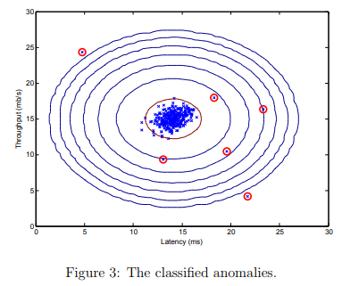
• Once you have completed the code in selectThreshold.m, the next step in ex8.m will run your anomaly detection code and circle the anomalies in the plot (Figure 3).

• Test 2a (Select threshold):
  input:
  [epsilon F1] = selectThreshold([1 0 0 1 1]', [0.1 0.2 0.3 0.4 0.5]')
  output:
  epsilon =  0.40040
  F1 =  0.57143
  

• The last part of the script ex8.m will run the anomaly detection algorithm you implemented on a more realistic and much harder dataset.




• In this dataset, each example is described by 11 features, capturing many more properties of your compute servers.




• The script will use your code to estimate the Gaussian parameters (µ_i and σ²_i), evaluate the probabilities for both the training data X from which you estimated the Gaussian parameters, and do so for the the cross-validation set Xval.




• Finally, it will use selectThreshold to find the best threshold ε. You should see a value epsilon of about 1.38e-18, and 117 anomalies found.