Introductory Video

• The Machine Learning course includes several programming assignments which you’ll need to finish to complete the course. The assignments require the Octave scientific computing language.




• Octave is a free, open-source application available for many platforms. It has a text interface and an experimental graphical one. Octave is distributed under the GNU Public License, which means that it is always free to download and distribute.




• Use Download to install Octave for windows. "Warning: Do not install Octave 4.0.0";




• Installing Octave on GNU/Linux : On Ubuntu, you can use: sudo apt-get update && sudo apt-get install octave. On Fedora, you can use: sudo yum install octave-forge

• In this exercise, you will implement Recommender Systems.




• Files included in this exercise can be downloaded here ⇒ : Download

• In this part of the exercise, you will implement the collaborative filtering learning algorithm and apply it to a dataset of movie ratings (MovieLens 100k Dataset from GroupLens Research).




• This dataset consists of ratings on a scale of 1 to 5. The dataset has n_u = 943 users, and n_m = 1682 movies.




• For this part of the exercise, you will be working with the script ex8_cofi.m.




• In the next partsof this exercise, you will implement the function cofiCostFunc.m that computes the collaborative fitlering objective function and gradient.




• After implementing the cost function and gradient, you will use fmincg.m to learn the parameters for collaborative filtering.

• The first part of the script ex8_cofi.m will load the dataset ex8_movies.mat, providing the variables Y and R in your Octave/MATLAB environment.




• The matrix Y (a_num_movies × num_users matrix) stores the ratings y^(i,j) (from 1 to 5). The matrix R is an binary-valued indicator matrix, where R(i, j) = 1 if user j gave a rating to movie i, and R(i, j) = 0 otherwise.




• The objective of collaborative filtering is to predict movie ratings for the movies that users have not yet rated, that is, the entries with R(i, j) = 0.




• This will allow us to recommend the movies with the highest predicted ratings to the user.




• To help you understand the matrix Y, the script ex8_cofi.m will compute the average movie rating for the first movie (Toy Story) and output the average rating to the screen.




• Throughout this part of the exercise, you will also be working with the matrices, X and Theta:




• 




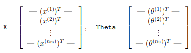
• The i-th row of X corresponds to the feature vector x⁽ⁱ⁾ for the i-th movie, and the j-th row of Theta corresponds to one parameter vector θ^(j) , for the j-th user.




• Both x⁽ⁱ⁾ and θ^(j) are n-dimensional vectors. For the purposes of this exercise, you will use n = 100, and therefore, x⁽ⁱ⁾ ∈ R¹⁰⁰ and θ^(j) ∈ R¹⁰⁰.




• Correspondingly, X is a n_m × 100 matrix and Theta is a n_u × 100 matrix

• Now, you will start implementing the collaborative filtering learning algorithm.




• You will start by implementing the cost function (without regularization).




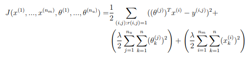
• The collaborative filtering algorithm in the setting of movie recommendations considers a set of n-dimensional parameter vectors x⁽¹⁾, ..., x^(n_m) and θ⁽¹⁾, ..., θ^(n_u) , where the model predicts the rating for movie i by user j as y^(i,j) = \( (θ^{(j)})^T x^{(i)} \). Given a dataset that consists of a set of ratings produced by some users on some movies, you wish to learn the parameter vectors x⁽¹⁾, ..., x^(n_m) and θ⁽¹⁾, ..., θ^(n_u) that produce the best fit (minimizes the squared error).




• You will complete the code in cofiCostFunc.m to compute the cost function and gradient for collaborative filtering.




• Note that the parameters to the function (i.e., the values that you are trying to learn) are X and Theta.




• In order to use an off-the-shelf minimizer such as fmincg, the cost function has been set up to unroll the parameters into a single vector params.




• You had previously used the same vector unrolling method in the neural networks programming exercise

• The collaborative filtering cost function (without regularization) is given by




• 




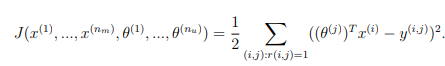
• You should now modify cofiCostFunc.m to return this cost in the variable J. Note that you should be accumulating the cost for user j and movie i only if R(i, j) = 1.




• After you have completed the function, the script ex8_cofi.m will run your cost function. You should expect to see an output of 22.22.




• Implementation Note: We strongly encourage you to use a vectorized implementation to compute J, since it will later by called many times by the optimization package fmincg.




• As usual, it might be easiest to first write a non-vectorized implementation (to make sure you have the right answer), and the modify it to become a vectorized implementation (checking that the vectorization steps don’t change your algorithm’s output).




• To come up with a vectorized implementation, the following tip might be helpful: You can use the R matrix to set selected entries to 0.




• For example, R .* M will do an element-wise multiplication between M and R; since R only has elements with values either 0 or 1, this has the effect of setting the elements of M to 0 only when the corresponding value in R is 0.




• Hence, sum(sum(R.*M)) is the sum of all the elements of M for which the corresponding element in R equals 1.

• R: a matrix of observations (binary values). Dimensions are (movies x users)




• Y: a matrix of movie ratings: Dimensions are (movies x users)




• X: a matrix of movie features (0 to 5): Dimensions are (movies x features)




• Theta: a matrix of feature weights: Dimensions are (users x features)




• Compute the predicted movie ratings for all users using the product of X and Theta. A transposition may be needed.




• Dimensions of the result should be (movies x users).




• Compute the movie rating error by subtracting Y from the predicted ratings.




• Compute the "error_factor"my multiplying the movie rating error by the R matrix. The error factor will be 0 for movies that a user has not rated. Use the type of multiplication by R (vector or element-wise) so the size of the error factor matrix remains unchanged (movies x users).




• Calculate the cost: Using the formula given above to compute the unregularized cost as a scaled sum of the squares of all of the terms in error_factor. The result should be a scalar.

• input:
  params = [ 1:14 ] / 10;
  Y = magic(4);
  Y = Y(:,1:3);
  R = [1 0 1; 1 1 1; 0 0 1; 1 1 0] > 0.5;     % R is logical
  num_users = 3;
  num_movies = 4;
  num_features = 2;
  lambda = 0;
  J = cofiCostFunc(params, Y, R, num_users, num_movies, num_features, lambda)
  output:
  J =  311.63    
  

• Now, you should implement the gradient (without regularization). Specifically, you should complete the code in cofiCostFunc.m to return the variables X_grad and Theta_grad.




• Note that X_grad should be a matrix of the same size as X and similarly, Theta grad is a matrix of the same size as Theta.




• The gradients of the cost function is given by:




• 




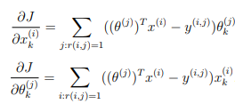
• Note that the function returns the gradient for both sets of variables by unrolling them into a single vector.




• After you have completed the code to compute the gradients, the script ex8_cofi.m will run a gradient check (checkCostFunction) to numerically check the implementation of your gradients (This is similar to the numerical check that you used in the neural networks exercise).




• If your implementation is correct, you should find that the analytical and numerical gradients match up closely.




• Implementation Note: You can get full credit for this assignment without using a vectorized implementation, but your code will run much more slowly (a small number of hours), and so we recommend that you try to vectorize your implementation.




• To get started, you can implement the gradient with a for-loop over movies (for computing \( \frac{\partial J}{\partial x^{(i)}_k} \) ) and a for-loop over users (for computing \( \frac{\partial J}{\partial \theta^{(j)}_k} \) ).




• When you first implement the gradient, you might start with an unvectorized version, by implementing another inner for-loop that computes each element in the summation.




• After you have completed the gradient computation this way, you should try to vectorize your implementation (vectorize the inner for-loops), so that you’re left with only two for-loops (one for looping over movies to compute \( \frac{\partial J}{\partial x^{(i)}_k} \) for each movie, and one for looping over users to compute \( \frac{\partial J}{\partial \theta^{(j)}_k} \) for each user).




• Implementation Tip: To perform the vectorization, you might find this helpful: You should come up with a way to compute all the derivatives associated with x⁽ⁱ⁾₁, x⁽ⁱ⁾₂, . . . , x⁽ⁱ⁾_n (i.e., the derivative terms associated with the feature vector x⁽ⁱ⁾ ) at the same time. Let us define the derivatives for the feature vector of the i-th movie as:




• 




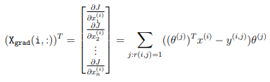
• To vectorize the above expression, you can start by indexing into Theta and Y to select only the elements of interests (that is, those with r(i, j) = 1).




• Intuitively, when you consider the features for the i-th movie, you only need to be concern about the users who had given ratings to the movie, and this allows you to remove all the other users from Theta and Y. Concretely, you can set idx = find(R(i, :)==1) to be a list of all the users that have rated movie i. This will allow you to create the temporary matrices Theta_temp = Theta(idx, :) and Y_temp = Y(i, idx) that index into Theta and Y to give you only the set of users which have rated the i-th movie. This will allow you to write the derivatives as:




• X_grad(i, :) = (X(i, :) ∗ Theta^T_temp − Y_temp) ∗ Theta_temp.




• (Note: The vectorized computation above returns a row-vector instead.) After you have vectorized the computations of the derivatives with respect to x⁽ⁱ⁾ , you should use a similar method to vectorize the derivatives with respect to θ^(j) as well.

• The X gradient is the product of the error factor and the Theta matrix. The sum is computed automatically by the vector multiplication. Dimensions are (movies x features)




• The Theta gradient is the product of the error factor and the X matrix. A transposition may be needed. The sum is computed automatically by the vector multiplication. Dimensions are (users x features)

• input:
  params = [ 1:14 ] / 10;
  Y = magic(4);
  Y = Y(:,1:3);
  R = [1 0 1; 1 1 1; 0 0 1; 1 1 0] > 0.5;     % R is logical
  num_users = 3;
  num_movies = 4;
  num_features = 2;
  lambda = 0;
  [J, grad] = cofiCostFunc(params, Y, R, num_users, num_movies, num_features, lambda)
  
  output:
  J =  311.63
  
  grad =
    -16.1880
    -23.5440
     -5.1590
    -14.9720
    -21.4380
    -30.4620
     -6.5660
    -19.5440
     -3.4230
     -7.0280
     -3.4140
    -12.2590
    -16.0600
     -9.7420
  

• The cost function for collaborative filtering with regularization is given by




• 




• You should now add regularization to your original computations of the cost function, J. After you are done, the script ex8_cofi.m will run your regularized cost function, and you should expect to see a cost of about 31.34.

• Using the formula given to compute the regularization term as the scaled sum of the squares of all terms in Theta and X. The result should be a scalar. Note that for Recommender Systems there are no bias terms, so regularization should include all columns of X and Theta.




• Add the regularized and un-regularized cost terms.




• Test your code, then submit this portion.

• input:
  params = [ 1:14 ] / 10;
  Y = magic(4);
  Y = Y(:,1:3);
  R = [1 0 1; 1 1 1; 0 0 1; 1 1 0] > 0.5;     % R is logical
  num_users = 3;
  num_movies = 4;
  num_features = 2;
  lambda = 6;
  J = cofiCostFunc(params, Y, R, num_users, num_movies, num_features, lambda)
  
  output:
  J =  342.08
  

• Now that you have implemented the regularized cost function, you should proceed to implement regularization for the gradient.




• You should add to your implementation in cofiCostFunc.m to return the regularized gradient by adding the contributions from the regularization terms.




• Note that the gradients for the regularized cost function is given by:




• 




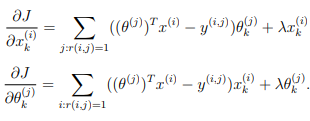
• This means that you just need to add λx⁽ⁱ⁾ to the X grad(i,:) variable described earlier, and add λθ^(j) to the Theta grad(j,:) variable described earlier.




• After you have completed the code to compute the gradients, the script ex8_cofi.m will run another gradient check (checkCostFunction) to numerically check the implementation of your gradients.

• The X gradient regularization is the X matrix scaled by lambda.




• The Theta gradient regularization is the Theta matrix scaled by lambda.




• Add the regularization terms to their unregularized values.




• Test your code, then submit this portion

• input:
  params = [ 1:14 ] / 10;
  Y = magic(4);
  Y = Y(:,1:3);
  R = [1 0 1; 1 1 1; 0 0 1; 1 1 0] > 0.5;     % R is logical
  num_users = 3;
  num_movies = 4;
  num_features = 2;
  lambda = 6;
  [J, grad] = cofiCostFunc(params, Y, R, num_users, num_movies, num_features, lambda)
  output:
  J =  342.08
  
  grad =
    -15.5880
    -22.3440
     -3.3590
    -12.5720
    -18.4380
    -26.8620
     -2.3660
    -14.7440
      1.9770
     -1.0280
      3.1860
     -5.0590
     -8.2600
     -1.3420
  

• input:
  params = [ 1:14 ] / 10;
  Y = magic(4);
  Y = Y(:,1:3);
  R = [1 0 1; 1 1 1; 0 0 0; 1 1 0] > 0.5;     % R is logical
  num_users = 3;
  num_movies = 4;
  num_features = 2;
  lambda = 6;
  [J, grad] = cofiCostFunc(params, Y, R, num_users, num_movies, num_features, lambda)
  output:
  J =  331.08
  
  grad =
    -15.5880
    -22.3440
      1.8000
    -12.5720
    -18.4380
    -26.8620
      4.2000
    -14.7440
      1.9770
     -1.0280
      4.5930
     -5.0590
     -8.2600
      1.9410
  

• After you have finished implementing the collaborative filtering cost function and gradient, you can now start training your algorithm to make movie recommendations for yourself.




• In the next part of the ex8_cofi.m script, you can enter your own movie preferences, so that later when the algorithm runs, you can get your own movie recommendations!




• We have filled out some values according to our own preferences, but you should change this according to your own tastes.




• The list of all movies and their number in the dataset can be found listed in the file movie_idx.txt.




• 




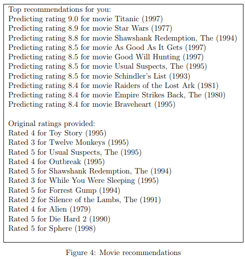
• After the additional ratings have been added to the dataset, the script will proceed to train the collaborative filtering model. This will learn the parameters X and Theta. To predict the rating of movie i for user j, you need to compute (\( (θ^{(j)})^T x^{(i)} \).




• The next part of the script computes the ratings for all the movies and users and displays the movies that it recommends (Figure 4), according to ratings that were entered earlier in the script.




• Note that you might obtain a different set of the predictions due to different random initializations.