Dynamic Programming - Optimal Binary search Tree
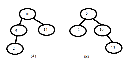
Construct a Optimal binary search tree of elements { 10 , 5 , 15, 2} for minimizing the access time. (Condition of BST is that root should be greater than left sub tree and less than right sub tree).
Now in the above two tree structures I have to access the element 10 and 5. The condition given to me is 10 is accessed once and 5 is accessed 4 times. The cost of one comparison is 1 nit so for tree A. We get:
1 * 1 + 2 * 4 = 9 units as cost of access. This is because 10 is the root element and it is accessed once and to access it we need only one comparison i.e. at position of root. But to access 5 we need two comparisons one at root and then at left sub tree. And this 2 comparisons are to be done 4 times.
For the second tree structure having the same access rates and cost we get 2 * 1 + 1 * 4 = 6; Therefore having an optimal binary search tree would lead to savings in cost.
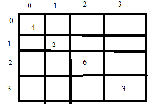
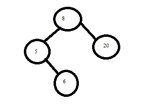
Consider the array of elements A = {5, 6, 8, 20} and corresponding accessing times is 4, 2, 6, 3. Now we have to create an optimal binary search tree to minimize the cost.
Step 1: We start with the diagonal elements. Assuming the matrix name is A then to fill position A[0,0] is like assuming the BST has only one element and that element is A[0] and we have to access it so what is the cost. So we know that A[0] is 5 and it is accessed 4 time so total cost is 4. A[0,0] = 4. Similarly filling all elements on the diagonal.
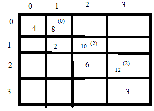
For position A[0,1] the intuition is: We now have two elements A[0], A[1] and now we need to create an optimal BST so which is the root that gives us minimum cost. We get that two cases:
Case 1: If A[0] is root then A[1] becomes right sub tree so we get cost of access as = 4 * 1 + 2 * 2 = 8
case 2: If A[1] is root then A[0] becomes left sub tree so we get cost of access as = 2 * 2 + 4 * 2 = 12
Therefore we select case 1 and put 8(0) in A[0,1] to indicate that cost of having A[0] as root is 8 and this is the minimum cost possible.
Using above procedure we repeat for A[1,2] and A[2,3] and get values 10(2) and 12(2) respectively.
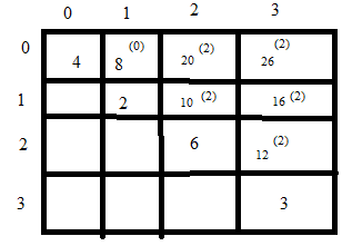
For the elements A[0,2] we have to solve three cases:
Case 1: Put A[0] as root and then we have A[1] and A[2] as sub elements of A[0]. This gives us minimum access of 10.
Case 2: Put A[1] as root and then we have A[0] and A[2] as sub elements of A[1]. This gives us minimum access of 10.
Case 3: Put A[2] as root and then we have A[1] and A[2] as sub elements of A[2]. This gives us minimum access of 8.
A second shorter way for finding A[0,2] = access(0) + access (1) + access(2) + min \( \left\{\begin{matrix} Root(0) = 10\\ Root(1) = 10\\ Root(2) = 8 \end{matrix}\right. \)
Here access(0) is cost of accessing element A[0] i.e. 5 so we write 4 and so on. Root(0) is A(1,2) { With A[0] as root what is access time for different trees obtained from combination A[1], A[2] } and Root(2) is A(0,1) are obtained from above figure. Access(0,2) is obtained as Access(0,0) + Access(2,2). So among the three conditions the minimum is 8(2). Using this we can also find element A[1,3] which we get as 16(2).
A[0,3] = access(0) + access (1) + access(2) + access(3) + min \( \left\{\begin{matrix} Root(0) = 16\\ Root(1) = 16\\ Root(2) = 11\\ Root(3) = 20 \end{matrix}\right. \)
To draw the final optimal binary tree we look at A[0,3] and it says 26(2) so we have root at 8 as it is A[2]. Then we get A[3] as right sub tree and for left tree we see A[0,1] and we have root as 0 there so we get final tree as.
Greedy Algorithms
A greedy algorithm always makes the choice that looks best at the moment. That is, it makes a locally optimal choice in the hope that this choice will lead to a globally optimal solution.
For many optimization problems, using dynamic programming to determine the best choices is overkill; simpler, more efficient algorithms will do.
Greedy Algorithms - An activity-selection problem
The goal of selecting a maximum-size set of mutually compatible activities. Suppose we have a set S = \( {a_1, a_2, ... ,a_n} \) of n proposed activities that wish to use a resource, such as a lecture hall, which can serve only one activity at a time. Each activity ai has a start time 's' and a finish time 'f' where 0 ≤ si ≤ fi ≤ ∞. Activities ai and aj are compatible if si ≥ fj OR sj ≥ fi . In the activity-selection problem, we wish to select a maximum-size subset of mutually compatible activities.
Solution:
Sort all activities in non - decreasing ( monotonically increasing ) order of the finish times.
Intuition suggests that we should choose an activity that leaves the resource available for as many other activities as possible. Now, of the activities we end up choosing, one of them must be the first one to finish. Our intuition tells us, therefore, to choose the activity in 'S' with the earliest finish time, since that would leave the resource available for as many of the activities that follow it as possible.
When the first activity finishes choose the next activity from amongst the remaining activities that fulfill the criterion (si ≥ fj).
Continue so on till the last activity is reached that can fulfill the criteria.
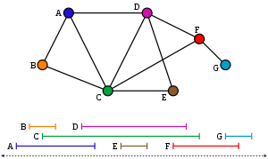
Greedy Algorithms - interval-graph coloring problem
Suppose that we have a set of activities to schedule among a large number of lecture halls, where any activity can take place in any lecture hall. We wish to schedule all the activities using as few lecture halls as possible. Give an efficient greedy algorithm to determine which activity should use which lecture hall.
Solution: This problem is also known as the interval-graph coloring problem. We can create an interval graph whose vertices are the given activities and whose edges connect incompatible activities. The smallest number of colors required to color every vertex so that no two adjacent vertices have the same color corresponds to finding the fewest lecture halls needed to schedule all of the given activities.
Maintain a set of free lecture halls F and currently busy lecture halls B. Sort the classes by start time.
For each new start time which you encounter, remove a lecture hall from F, schedule the class in that room, and add the lecture hall to B.
If F is empty, add a new, unused lecture hall to F. When a class finishes, remove its lecture hall from B and add it to F. Why this is optimal: Suppose we have just started using the mth lecture hall for the first time.
This only happens when ever classroom ever used before is in B. But this means that there are m classes occurring simultaneously, so it is necessary to have m distinct lecture halls in use.
Dynamic Programming - 0/1 Knapsack problem
Given a set of items, each with a weight and a value, determine the number of each item to include in a collection so that the total weight is less than or equal to a given limit and the total value is as large as possible.
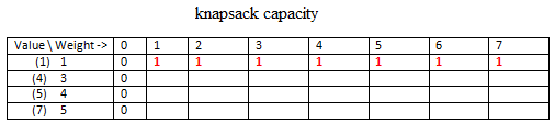
So we have a set of items and their corresponding weights and values as given in the table. Also the total weight of the knapsack is given to as as shown. Now since we can either take the item or reject it we have 0/1 case. When we can split the item then we have a case of "Fractional Knapsack whose greedy solution is possible.
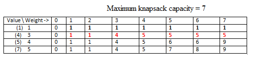
So initially we have a table with columns to indicate various ranges of knapsack weights i.e. from min to max so {0-7}. The left most columns indicate the item values and weights given in this question.
So in the first step the column of knapsack weight = 0 has all rows set to 0. This means that when the knapsack has capacity = 0 kg, no matter how many items we have we cant take any.
Now the red entry indicate, when we have only 1 item (value=1) then with any capacity of knapsack we can have value only 1 (maximum).
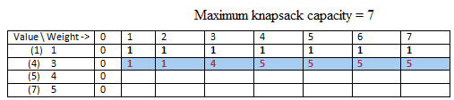
In the second row, we have two items and now we have to maximize the value in the knapsack with these two items. For elements T[0,1] and T[0,2] we put 1. This is because the capacity of the knapsack is 1 and 2 respectively and we can accommodate item 2, so we get max value in knapsack as 1. But for T[0,3] the max possible weight in knapsack is 3 and so we remove item 1 and put item 2 as it gives more value. T[0,4] we can accomodate both items together and so value = 5.
Continuing in this manner we get the full solution.

Pseudocode - 0/1 Knapsack problem
// Input:
// Values (stored in array v)
// Weights (stored in array w)
// Number of distinct items (n)
// Knapsack capacity (W)
for j from 0 to W do:
m[0, j] := 0
for i from 1 to n do:
for j from 0 to W do:
if w[i] > j then:
m[i, j] := m[i-1, j]
else:
m[i, j] := max(m[i-1, j], m[i-1, j-w[i]] + v[i])
Greedy Algorithms - Fractional Knapsack problem
Given weights and values of n items, we need put these items in a knapsack of capacity W to get the maximum total value in the knapsack.
A brute-force solution would be to try all possible subset with all different fraction.
An efficient solution is to use Greedy approach. The basic idea of greedy approach is to calculate the ratio value/weight for each item and sort the item on basis of this ratio. Then take the item with highest ratio and add them until we can’t add the next item as whole and at the end add the next item as much as we can.
Thus, by sorting the items by value per pound, the greedy algorithm runs in O(n lg n) time.
Greedy Algorithms - Set Cover problem
Given a universe U of n elements, a collection of subsets of U say S = \( {S_1 , S_2 …,S_m } \) where every subset \( S_i \) has an associated cost. Find a minimum cost sub collection of S that covers all elements of U.
Example: U = {1,2,3,4,5} S = \( {S_1 , S_2 …,S_m } \)
S1 = {4,1,3}, Cost(1) = 5 S2 = {2,5}, Cost(S 2) = 10 S3 = {1,4,3,2}, Cost(S3) = 3
Output: Minimum cost of set cover is 13 and set cover is {S2, S3} There are two possible set covers {S1 , S2 } with cost 15 and {S2 , S3 } with cost 13.
Set Cover problem
Set Cover is NP-Hard:There is no polynomial time solution available for this problem as the problem is a known NP- Hard problem. There is a polynomial time Greedy approximate algorithm, the greedy algorithm provides a Log n approximate algorithm.
Let U be the universe of elements, S = \( {S_1 , S_2 …,S_m } \) be collection of subsets of U and Cost(S1), C(S2), … Cost(Sm) be costs of subsets.
Let I represent set of elements included so far. Initialize I = {}
Do following while I is not same as U.
Find the set Si in \( {S_1 , S_2 …,S_m } \) whose cost effectiveness is smallest, i.e., the ratio of cost C(Si) and number of newly added elements is minimum. Basically we pick the set for which following value is minimum. Cost(Si) / |Si - I|
Add elements of above picked Si to I, i.e., I = I ∪ Si
Set Cover problem - Example
First iteration: I = {}, S1 = {4,1,3}, S2 = {2,5}, S3 = {1,4,3,2}
The per new element cost for S1 = Cost(S1)/|S1 – I| = 5/3
The per new element cost for S2 = Cost(S2 )/|S2 – I| = 10/2
The per new element cost for S3 = Cost(S3 )/|S3 – I| = 3/4
Since S3 has minimum value S3 is added, I becomes {1,4,3,2}.
Second Iteration: I = {1,4,3,2}
The per new element cost for S1 = Cost(S1 )/|S1 – I| = 5/0 Note that S1 doesn’t add any new element to I.
The per new element cost for S2 = Cost(S2 )/|S2 – I| = 10/1 Note that S2 adds only 5 to I. The greedy algorithm provides the optimal solution for above example, but it may not provide optimal solution all the time.
Set Cover problem - Example
S1 = {1, 2}
S2 = {2, 3, 4, 5}
S3 = {6, 7, 8, 9, 10, 11, 12, 13}
S3 = {1, 3, 5, 7, 9, 11, 13}
S5 = {2, 4, 6, 8, 10, 12, 13}
Let the cost of every set be same.
The greedy algorithm produces result as {S3 , S2 , S1}
The optimal solution is {S4 , S5 }
Solved Question Papers
Q.5 List1(Gate 2015 Set1)
| LIST 1 | LIST 2 |
|---|---|
| Prim’s algorithm for minimum spanning tree | Backtracking |
| Floyd-Warshall algorithm for all pairs shortest paths | Greedy method |
| Mergesort | Dynamic programming |
| Hamiltonian circuit | Divide and conquer |
Codes
A B C D
3 2 4 1
1 2 4 3
2 3 4 1
2 1 3 4
Ans (C)
Prim’s Algorithm is a greedy algorithm where greedy choice is to pick minimum weight edge from cut that divides already picked vertices and vertices yet to be picked. Floyd-Warshall algorithm for all pairs shortest paths is a Dynamic Programming algorithm where we keep updating the distance matrix in bottom up manner. Merge Sort is clearly divide and conquer which follows all steps of divide and conquer. It first divides the array in two halves, then conquer the two halves and finally combines the conquered results. Hamiltonian circuit is a NP complete problem, that can be solved using Backtracking.
Solved Question Papers
Q.Given below are some algorithms, and some algorithm design paradigms.
List-I
A. Dijkstra’s Shortest Path
B. Floyd-Warshall algorithm to compute all pairs shortest path
C. Binary search on a sorted array
D. Backtracking search on a graph
List-II
1. Divide and Conquer
2. Dynamic Programming
3. Greedy design
4. Depth-first search
5. Breadth-first search
Match the above algorithms on the left to the corresponding design paradigm they follow
Codes:
A B C D
(a) 1 3 1 5
(b) 3 3 1 5
(c) 3 2 1 4
(d) 3 2 1 5
(GATE 2015 SET B)
a
b
c
d
Ans . C
Q. What is the value returned by the function f given below when n=100 ? (UGC 2016 Paper 2)
int f (int n)
{
  if (n==0) then return n;
  else
  return n + f(n-2);
}
-
2550
-
2556
-
5220
-
5520
Ans. 1
Explanation:-
The given function is a recursive function which takes starting value as 100. It keeps on adding the present value and the value obtained by calling the function f(n-2) where n is current value.
It stops at n=0 where it returns 0.
As a result, it forms an AP starting with first term as 2 and last term as 100 with 2 common difference and total terms as 50.
So applying Sum of AP, we get :- S= (n*(a+l))/2 = (50*(2+100))/2 = 2550.
Q. Consider the following operation along with Enqueue and Dequeue operations on queues, where k is a global parameter
MultiDequeue(Q){
   m = k
   while (Q is not empty and m  > 0) {
      Dequeue(Q)
      m = m - 1
   }
}
What is the worst case time complexity of a sequence of n MultiDequeue() operations on an initially empty queue?
-
Θ(n)
-
Θ(n + k)
-
Θ(nk)
-
Θ(n2)
Ans. 2
Since the queue is empty initially, the condition of while loop never becomes true. So the time complexity is Θ(n)
Q. What is the time complexity of Bellman-Ford single-source shortest path algorithm on a complete graph of n vertices?
-
Θ(n2)
-
Θ(n2 logn)
-
Θ(n3)
-
Θ(n3 logn)
Ans. 3
Time complexity of Bellman-Ford algorithm is Θ(VE) where V is number of vertices and E is number edges . If the graph is complete, the value of E becomes Θ(V2). So overall time complexity becomes Θ(V3)