Shortest Path Algorithms
BELMANFORD(G,w)
for v in V
v.d = ∞
v.π = null
s.d = 0 // source node
for i = 1 to |v| - 1
for (u,v) ∈ E
relax(u,v,w)
for (u,v) in E
if v.d > u.d + w(u,v)
report negative cycle exists
RELAX(u,v)
if v.d > u.d + w(u,v)
v.d = u.d + w(u,v)
v.π = u;
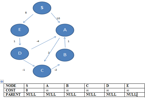
Shortest Path Algorithms - BELMANFORD
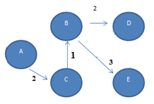
STEP 1: Initialization of source node to 0 and all other nodes to infinity with parents = NULL for all except source {S}
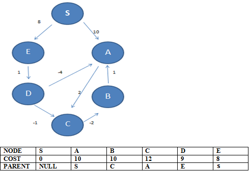
From S we take the outgoing edges to E and A. Then we update the weights as 8 and 10 respectively as it is less than their original weights i.e. ∞ We also update parents to S from NULL for both.
Then from A we take the outgoing edge to C and update weight and parent to 12 (10+2) and A. We update weight to 12 as we take total 12 units to reach C from source S and intermediate step A.
We move on to B, but B has cost ∞ so we skip it.
Next is C, we see outgoing edge to B and update cost and parent as 10(12-2) and C respectively.
We move on to D, but D has cost ∞ so we skip it.
We then move to E, and examine its outgoing edge to D. We update D to cost 9(8+1) and parent E.
FIRST ITERATION OVER
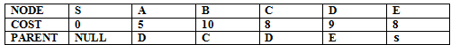
STEP 2:
We start with S but the edges show no improvement and so table isnt updates. Same is with A, B, C.
Examining D and its outgoing edges to A and C we get an improvement and so we update cost as 5 and 8 and parents as D
We move to D but there is no improvement.
SECOND ITERATION IS OVER
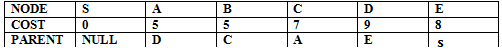
STEP 3:
In iteration 3 , the changes made are only by node A to C whose cost is now 7. Then when we examine C, the outgoing edge to B shows reduction in cost to 5 from 10.
STEP 4: NO UPDATION
STEP 5: NO UPDATION
The Bellman-Ford algorithm runs in time O(VE), since the initialization takes Θ(V) time, each of the |V|-1 passes over the edges and takes Θ(E) time, and the "for loop" takes O(E) time.
Shortest Path Algorithms - Dijkstra's Algorithm
DIJKSTRA(G,w,s) // s is source, w is weight
for v in V
v.d = ∞
v.π = null
s.d = 0 // source node
s = φ
Q = V - S
while Q ≠ φ
u = extract-min(Q)
s = s ∪ {u}for each vertex x ∈ adj[u]
relax(u,v,w)
RELAX(u,v)
if v.d > u.d + w(u,v)
v.d = u.d + w(u,v)
v.π = u;
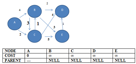
Dijkstra's Algorithm Example
STEP 1: Initialization of source A to 0 and others to ∞ with parents NULL
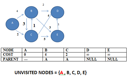
Examine outgoing edges of A to B and C and update their original weights ∞ to new weights 4 and 2 with parent A. We also remove A from the set of unvisited nodes.
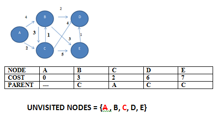
STEP 2: Then we choose the node with the lowest weight amongst the unvisited nodes i.e. C.
From C we update the nodes B,D and E with new weights and change their parent node as shown below.
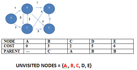
STEP 3: Then we choose the node with the lowest weight amongst the unvisited nodes i.e. B.
We update the values of D and E as shown below.
STEP 4: CHOOSE D; NO UPDATES
STEP 5: CHOOSE E; NO UPDATES. So we get the final tree as below.
All Pair Shortest Path
We can solve an all-pairs shortest-paths problem by running a single-source shortest-paths algorithm |V| times, once for each vertex as the source. If all edge weights are nonnegative, we can use Dijkstra’s algorithm.
If we use the linear-array implementation of the min-priority queue, the running time is \( O(V^3) \).
If the graph has negative-weight edges, we cannot use Dijkstra’s algorithm. Instead, we must run the slower Bellman-Ford algorithm once from each vertex. The resulting running time is \( O(V^4) \)
Floyd Warshall Algorithm
FLOYD-WARSHALL(G)
let V be the number of vertices in the graph
let dist be a V * V array of minimum distances and p be V * V array to store parent node value.
for each vertex v
dist[v][v] <- 0
for each edge (u,v)
dist[u][v] <- weight(u,v)
for k = 1 to V
for i = 1 to V
for j = 1 to V
if dist[i][j] > dist[i][k] + dist[k][j]
dist[i][j] = dist[i][k] + dist[k][j]
p[i][j] = p[k][j]
end if
Floyd Warshall Algorithm - Working
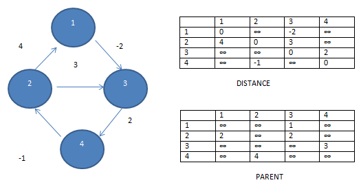
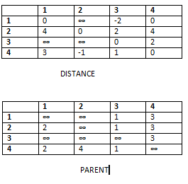
STEP 1: Initialize the dist matrix with weights and ∞ in places where edges are absent. Also all cells with A[i][i] should be zero. Fill p matrix with parent nodes if edge available OR ∞ for places with no edges.
For k = 0, i = 0, j = 0 to 3
d[0][0] > d[0][0] + d[0][0]
d[0][1] > d[0][0] + d[0][1]
d[0][2] > d[0][0] + d[0][2]
d[0][3] > d[0][0] + d[0][3]
Above all cases give condition as false so no update to any table
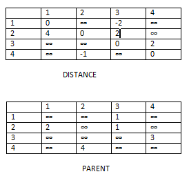
For k = 0, i = 1, j = 0 to 3
d[1][0] > d[1][0] + d[0][0]
d[1][1] > d[1][0] + d[0][1]
d[1][2] > d[1][0] + d[0][2]
d[1][3] > d[1][0] + d[0][3]
Above all cases iteration 3 gives condition true and we have to modify entry d[1][2] = 2 and p[1][2] = 1.
For k = 0, i = 2, j = 0 to 3
d[2][0] > d[2][0] + d[0][0]
d[2][1] > d[2][0] + d[0][1]
d[2][2] > d[2][0] + d[0][2]
d[2][3] > d[2][0] + d[0][3]
Above all cases give condition as false so no update to any table
For k = 0, i = 3, j = 0 to 3
d[3][0] > d[3][0] + d[0][0]
d[3][1] > d[3][0] + d[0][1]
d[3][2] > d[3][0] + d[0][2]
d[3][3] > d[3][0] + d[0][3]
Above all cases give condition as false so no update to any table
STEP 2: K is incremented to 1
For k = 1, i = 0, j = 0 to 3
d[0][0] > d[0][1] + d[1][0]
d[0][1] > d[0][1] + d[1][1]
d[0][2] > d[0][1] + d[1][2]
d[0][3] > d[0][1] + d[1][3]
Above all cases give condition as false so no update to any table
For k = 1, i = 1, j = 0 to 3
d[1][0] > d[1][1] + d[1][0]
d[1][1] > d[1][1] + d[1][1]
d[1][2] > d[1][1] + d[1][2]
d[1][3] > d[1][1] + d[1][3]
Above all cases give condition as false so no update to any table
For k = 1, i = 2, j = 0 to 3
d[2][0] > d[2][1] + d[1][0]
d[2][1] > d[2][1] + d[1][1]
d[2][2] > d[2][1] + d[1][2]
d[2][3] > d[2][1] + d[1][3]
Above all cases give condition as false so no update to any table
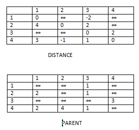
For k = 1, i = 3, j = 0 to 3
d[3][0] > d[3][1] + d[1][0]
d[3][1] > d[3][1] + d[1][1]
d[3][2] > d[3][1] + d[1][2]
d[3][3] > d[3][1] + d[1][3]
For 1st iteration the condition is true and we modify d[3][0] = 3 and p[3][0] = 2. For 3rd iteration the modification is of d[3][2] = 1 and p[3][2] = 1.
STEP 3: K is incremented to 2
For k = 2, i = 0, j = 0 to 3
d[0][0] > d[0][2] + d[2][0]
d[0][1] > d[0][2] + d[2][1]
d[0][2] > d[0][2] + d[2][2]
d[0][3] > d[0][2] + d[2][3]
Modification is at d[0][3] and we put d[0][3] = 0, p[0][3] = 3.
For k = 2, i = 1, j = 0 to 3
d[1][0] > d[1][2] + d[2][0]
d[1][1] > d[1][2] + d[2][1]
d[1][2] > d[1][2] + d[2][2]
d[1][3] > d[1][2] + d[2][3]
Modification is at d[1][3] and we put d[1][3] = 0, p[1][3] = 3.
For k = 2, i = 2, j = 0 to 3
d[2][0] > d[2][2] + d[2][0]
d[2][1] > d[2][2] + d[2][1]
d[2][2] > d[2][2] + d[2][2]
d[2][3] > d[2][2] + d[2][3]
Above all cases give condition as false so no update to any table
For k = 3, i = 3, j = 0 to 3
d[3][0] > d[3][3] + d[3][0]
d[3][1] > d[3][3] + d[3][1]
d[3][2] > d[3][3] + d[3][2]
d[3][3] > d[3][3] + d[3][3]
Above all cases give condition as false so no update to any table.
STEP 3: K is incremented to 3
For k = 3, i = 0, j = 0 to 3
d[0][0] > d[0][3] + d[3][0]
d[0][1] > d[0][3] + d[3][1]
d[0][2] > d[0][3] + d[3][2]
d[0][3] > d[0][3] + d[3][3]
Modification is at d[0][1] and we put d[0][1] = -1, p[0][1] = 4.
For k = 3, i = 1, j = 0 to 3
d[1][0] > d[1][3] + d[3][0]
d[1][1] > d[1][3] + d[3][1]
d[1][2] > d[1][3] + d[3][2]
d[1][3] > d[1][3] + d[3][3]
Above all cases give condition as false so no update to any table.
For k = 3, i = 2, j = 0 to 3
d[2][0] > d[2][3] + d[3][0]
d[2][1] > d[2][3] + d[3][1]
d[2][2] > d[2][3] + d[3][2]
d[2][3] > d[2][3] + d[3][3]
Modify d[2][0] as 5, p[2][0] as 2; d[2][1] = 1, p[2][1]= 4.
For k = 3, i = 3, j = 0 to 3
d[3][0] > d[3][3] + d[3][0]
d[3][1] > d[3][3] + d[3][1]
d[3][2] > d[3][3] + d[3][2]
d[3][3] > d[3][3] + d[3][3]
Above all cases give condition as false so no update to any table.
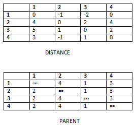
Time complexity = \( O(V^3) \)
Solved Question Papers
Q. What is the time complexity of Bellman-Ford single-source shortest path algorithm on a complete graph of n vertices? (GATE 2013 SET D)
\(\theta(n^{2})\)
\(\theta(n^2\log n)\)
\(\theta(n^3)\)
\(\theta(n^3\log n)\)
Ans . 3
Bellman-ford time complexity: \( \theta(\mid V\mid \times \mid E \mid)\)
For complete graph : \( \mid E\mid = \frac{n\left(n-1\right)}{2}\)
\( \mid V \mid = n\)
\( \theta ( n \times (\frac{n(n-1)}{2})) = \theta (n^{3}) \)
Q. Which of the following statement (s) is/are correct regarding Bellman-Ford shortest path algorithm? (GATE 2009)
P. Always find a negative weighted cycle, if one exists
Q. Finds whether any negative weighted cycle is reachable from the source.
(A) P only
(B) Both P and Q
(C) Q only
(D) Neither P nor Q
Ans . C
Bellman-Ford shortest path algorithm is a single source shortest path algorithm. So it can only find cycles which are reachable from a given source, not any negative weight cycle. Consider a disconnected graph where a negative weight cycle is not reachable from the source at all. If there is a negative weight cycle, then it will appear in shortest path as the negative weight cycle will always form a shorter path when iterated through the cycle again and again
Q. Which of the following statement(s)is / are correct regarding Bellman-Ford shortest path algorithm? P: Always finds a negative weighted cycle, if one exist s. Q: Finds whether any negative weighted cycle is reachable from the source. (GATE 2009)
P Only
Q Only
Both P and Q
Neither P nor Q
Ans: B
Que 5: Consider the directed graph shown in the figure below. There are multiple shortest paths between vertices S and T. Which one will be reported by Dijkstra's shortest path algorithm? Assume that, in any iteration, the shortest path to a vertex v is updated only when a strictly shorter path to v is discovered. (GATE 2016 SET B)
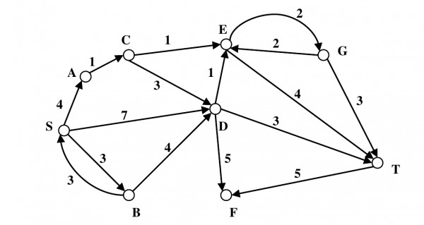
SDT
SBDT
SACDT
SACET
Ans . D
Let d[v] represent the shortest path distance computed from S Initially d[S]=0, d[A] = ∞ , d[B] = ∞,..........,d[T] = ∞
And let P[v] represent the predecessor of v in the shortest path from S to v and let P[v]=-1 denote that currently predecessor of v has not been computed
Let Q be the set of vertices for which shortest path distance has not been computed
Let W be the set of vertices for which shortest path distance has not been computed
So initially, Q = {S,A,B,C,D,E,F,G,T ,W} = ∅
We will use the following procedure Repeat until Q is empty
- u = choose a vertex from Q with minimum d[u] value
- Q = Q - u
- update all the adjacent vertices of u
- W = W U{u}
d[S] = 0, d[A] = ∞ , d[B] = ∞ , , d[T] = ∞
Iteration: 1
- u=S
- Q ={A,B,C,D,E,F,G,T}
- final values after adjustment d[S]=0, d[A]=4, d[B]=3, d[C]=∞, d{D]=7, d[E]=∞,........,d[T]=∞, P[A]=S, P[B]=S, P[C]=-1, P[D]=S, P[E]=-1,..............,P[T]=-1
- W={S}
Iteration: 2
- u=B
- Q = {A,C,D,E,F,G,T}
- final values after adjustment d[S]=0, d[A]=4, d[b]=3, d[C]=∞, d[D]=7, d[E]=∞,........,d[T]=&infin, P[A]=S, P[B]=S, P[C]=-1, P[D]=S, P[E]=-1,...........,P[T]=-1
- W = {S,B}
Iteration: 3
- u = A
- Q = {C,D,E,F,G,T}
- final values after adjustment d[S]=0, d[A]=4, d[B]=3, d[C]=5, d[D] =7, d[E]= ∞,........,P[A]=S, P[B]=S, P[C]=A, P[D]=S, P[E]=-1
- W = {S,B,A}
Iteration: 4
- u = C
- Q = {D, E, F, G, T}
- final values after adjustment d[S]=0, d[A]=4, d[B]=3, d[C]=5, d[D]=7, d[E]=6,....,d[T]= &nfin;, P[A]=S, P[B]=S, P[C]=A, P[D]=S, P[E]=C,......,P[T]=-1
- W = {S,B,A,C}
Iteration 5:
- u = E
- Q = {D, F, G, T}
- final values after adjustment d[S]=0, d[A]=4, d[B]=3, d[C]=5, d[D]=7, d[E]=6, d[F]=∞, d[G] = 8, d[T]=10, P[A]=S, P[B]=S, P[C]=A, P[D]=S, P[E]=C, P[F]=-1, P[G]=E, P[T]=E
- W = {S,B,A,C,E}
After iteration 5, we can observe that P[T]=E , P[E]=C , P[C]=A , P[A]=S, So the shortest path from S to T is SACET
Que 6: A list of n strings, each of length n, is sorted into lexicographic order using the merge-sort algorithm. The worst case running time of this computation is (GATE 2016 SET B)
O(n log n)
O(n2log n )
O(n2 + log n)
O(n2)
Ans . B
The height of the recursion tree using merge sort is logn and n2 comparisons are done at each level, where at most n pairs of strings are compared at each level and n comparisons are required to compare any two strings, So the worst case running time is O(n2 log n)