Algorithms and Complexity (Divide and Conquer) - Gate CSE

In divide-and-conquer, we solve a problem recursively, applying three steps at each level of the recursion:

Divide the problem into a number of sub-problems that are smaller instances of the same problem.

Conquer the sub-problems by solving them recursively. If the sub-problem sizes are small enough, however, just solve the sub-problems in a straightforward manner.

Combine the solutions to the sub-problems into the solution for the original problem.

When the sub-problems are large enough to solve recursively, we call that the recursive case. Once the sub-problems become small enough that we no longer recurse, we say that the recursion “bottoms out” and that we have gotten down to the base case.

Recurrences can take many forms. For example, a recursive algorithm might divide sub-problems into unequal sizes, such as a 2/3 to 1/3 split. If the divide and combine steps take linear time, such an algorithm would give rise to the recurrence

T(n) = T(2n/3) + T(n/3) + Θ(n)

Aim: To find the maximum subarray of the Array

Suppose we want to ﬁnd a maximum subarray of the subarray A[low...high]. Divide-and-conquer suggests that we divide the subarray into two subarrays of as equal size as possible. That is, we ﬁnd the midpoint, say mid, of the subarray, and consider the subarrays A[low..mid] and A[mid+1....high].
Any contiguous subarray A[i...j] of A[low...high] must lie in exactly one of the following places:

Entirely in the subarray A[low..mid],so that low ≤ i ≤ j ≤ mid

entirely in the subarray A[mid + 1...high],so that mid < i ≤ j ≤ high,or
crossing the midpoint, so that low ≤ i ≤ mid < j ≤ high.

Therefore, a maximum subarray of A[low...high] must lie in exactly one of these places. In fact, a maximum subarray of A[low...high] must have the greatest sum over all subarrays entirely in A[low...mid], entirely in A[mid + 1..high], or crossing the midpoint. We can ﬁnd maximum subarrays of A[low...mid] and A[mid+1...high] recursively, because these two subproblems are smaller instances of the problem of ﬁnding a maximum subarray.
Any subarray crossing the midpoint is itself made of two subarrays A[i...mid] and A[mid + 1...j],where low ≤ i ≤ mid and mid < j ≤ high. Therefore, we just need to ﬁnd maximum subarrays of the form A[i...mid] and A[mid+1..j] and then combine them.

Maximum Subarray Algorithm

FIND-MAX-CROSSING-SUBARRAY(A, low, mid, high)

```
left-sum = -∞
```
```
sum = 0
```
```
for i = mid downto low
```
```
     sum = sum + A[i]
```
```
     if sum > left-sum
```
```
        left-sum = sum
```
```
        max-left = i
```
```
right-sum = -∞
```
```
sum = 0
```
```
for j = mid + 1 to high
```
```
     sum = sum + A[j]
```
```
     if sum > right-sum
```
```
         right-sum = sum
```
```
         max-right = j
```

return (max-left, max-right, left-sum + right-sum)

Maximum Subarray Algorithm - Divide and Conquer

```
FIND-MAXIMUM-SUBARRAY(A, low, high)
```
```
if high == low
```

   return (low, high,A[low]) // base case: only one element

```
else mid = (low + high)/2
```

   (left-low,left-high, left-sum) = FIND-MAXIMUM-SUBARRAY(A, low, mid)

   (right-low, right-high, right-sum) = FIND-MAXIMUM-SUBARRAY(A, mid+1, high)

   (cross-low, cross-high, cross-sum) = FIND-MAX-CROSSING-SUBARRAY(A, low, mid, high)

   if left-sum > right-sum and left-sum > cross-sum

      return (left-low, left-high, left-sum)

   elseif right-sum > left-sum and right-sum > cross-sum

      return (right-low, right-high, right-sum)

   else return (cross-low, cross-high, cross-sum)

Q. What does FIND-MAXIMUM-SUBARRAY return when all elements of A are negative?

It will return the least negative position. As each of the cross sums are computed, the most positive one must have the shorest possible lengths.
The algoritm doesn't consider length zero sub arrays, so it must have length 1.

Q. Write pseudocode for the brute-force method of solving the maximum-subarray problem. Your procedure should run in Θ(n²) time.

Algorithm 1: Brute Force Algorithm to Solve Maximum Subarray Problem

```
left = 1
```
```
right = 1
```
```
max = A[1]
```
```
curSum = 0
```

for i = 1 to n do // Increment left end of subarray

```
   curSum = 0
```

   for j = i to n do // Increment right end of subarray

```
      curSum = curSum + A[j]
```
```
      if curSum > max then
```
```
         max = curSum
```
```
         left = i
```
```
         right = j
```
```
      end if
```
```
   end for
```
```
end for
```

Q. Develop a nonrecursive, linear-time algorithm for the maximum-subarray problem.

Algorithm 2: linear time maximum subarray(A)

```
M = - ∞
```
```
low_M, high_M  = null
```
```
M_r = 0
```
```
low_r = 1
```
```
for i from 1 to A.length do
```
```
    M_r + = A[i]
```
```
    if M_r > M then 
```
```
       low_M = low_r
```
```
       high_M = i
```
```
       M = M_r
```
```
    end if
```
```
    if M_r < 0 then
```
```
       M_r = 0
```
```
       low_r = i + 1
```
```
    end if
```
```
    return ( low_M, high_M, M  )
```
```
end for
```

If A = (a_ij) and B = (b_ij) are square n * n matrices, then in the product C = A . B,we define the entry (c_ij) for i, j = 1, 2 , ... , n by

\( c_{ij} = \sum_{k = 1}^{n} a_{ik} . b_{kj} \)

We must compute n² matrix entries, and each is the sum of n values. The following procedure takes n * n matrices A and B and multiplies them, returning their n * n product C. We assume that each matrix has an attribute rows, giving the number of rows in the matrix.

```
SQUARE-MATRIX-MULTIPLY(A,B)
```
```
n = A.rows
```
```
let C be a new n*n matrix
```
```
for i = 1 to n
```
```
   for j = 1 to n
```
```
       c_ij = 0
```
```
       for k = 1 to n
```
```
           c_ij = c_ij + (a_ik * b_kj)
```
```
return C
```

Time Complexity:Because each of the triply-nested for loops runs exactly 'n' iterations, and each execution of line 9 takes constant time, the SQUARE-MATRIX-MULTIPLY procedure takes Θ(n³) time.

To compute the matrix product C = A * B, we assume that n is an exact power of 2 in each of the n * n matrices.

```
Algorithm 3: Strassen(A, B)
```
```
if A.length == 1 then
```
```
   return A[1] . B[1]
```
```
end if
```
```
Let C be a new n by n matrix
```
```
A11 = A[1..n/2][1..n/2]
```
```
A12 = A[1...n/2][n/2 + 1...n]
```
```
A21 = A[n/2 + 1...n][1...n/2]
```
```
A22 = A[n/2 + 1...n][n/2 + 1...n]
```
```
B11 = B[1...n/2][1...n/2]
```
```
B12 = B[1...n/2][n/2 + 1...n]
```
```
B21 = B[n/2 + 1...n][1...n/2]
```
```
B22 = B[n/2 + 1...n][n/2 + 1...n]
```
```
S1= B12 + B22
```
```
S2= A11 + A12
```
```
S3= A21 + A22
```
```
S4= B21 - B11
```
```
S5= A11 + A22
```
```
S6= B11 + B22
```
```
S7= A12 - A22
```
```
S8= B21 + B22
```
```
S9= A11 - A21
```
```
S10= B11 + B12
```
```
P1 = Strassen(A11; S1)
```
```
P2 = Strassen(S2, B22)
```
```
P3 = Strassen(S3, B11)
```
```
P4 = Strassen(A22, S4)
```
```
P5 = Strassen(S5, S6)
```
```
P6 = Strassen(S7, S8)
```
```
P7 = Strassen(S9, S10)
```
```
C[1...n/2][1...n/2] = P5 + P4 - P2 + P6
```
```
C[1...n/2][n/2 + 1...n] = P1 + P2
```
```
C[n/2 + 1...n][1...n/2] = P3 + P4
```

C[n/2 + 1...n][n/2 + 1...n] = P5 + P1 - P3 - P7

```
return C
```

Time Complexity:Θ(n^2.81) time.

Let's use the iterative method to figure out the running time of merge_sort. We know that for Merge sort
T(1) = 1
T(n) = 2 T(n/2) + n
Starting with the iterative method, we can start expanding the time equation until we notice a pattern:

Solution:

```
T(n) = n + T(n/2)
```
```
     = n + n + T(n/4)
```
```
     = n + n + n + T(n/8)
```
```
     = n +  n + n + n + T(n/2⁴)
```
```
After 'k' iterations
```

     T(n) = n +  n + n + n + n + ... + T(n/2^k)

```
Assume  n=2^k then  k = lg n  and 
```
```
     T(n) = k * n + T(1)
```
```
     T(n) =  n lg n 
```

Q. Solve the recurrence using iteration method: T(n) = c + T(n/2)

```
T(n) = c + T(n/2)
```
```
     = c + c + T(n/4)
```
```
     = c + c + c + T(n/8)
```
```
     = c +  c + c + c + T(n/2⁴)
```
```
After 'k' iterations
```

     T(n) = c +  c + c + c + c + ... + T(n/2^k)

```
Assume  n=2^k then  k = lg n  and 
```
```
     T(n) = k * c + T(1)
```
```
     T(n) =  c lg n 
```

Q. Solve the recurrance using iteration method: T(n) = n + 2T(n/2)

```
T(n) = n + 2T(n/2)
```
```
     = n + 2(n/2 + 2T(n/4))
```
```
= n + n + 4T(n/4)
```
```
= n + n + 4(n/4 + 2T(n/8))
```
```
= n + n + n + 8T(n/8)
```
```
T(n) = 3n + 2³T(n/2³)
```
```
After 'k' iterations it is now:
```
```
T(n) = 3n + 2^kT(n/2^k)
```
```
Assume  n=2^k, k = lg n
```
```
= n lg n+ n T(1)
```
```
T(n) = O(nlgn)
```

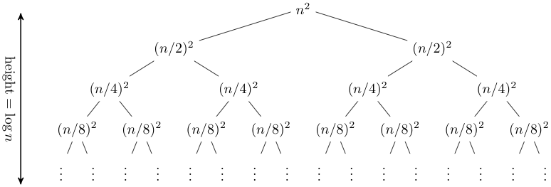
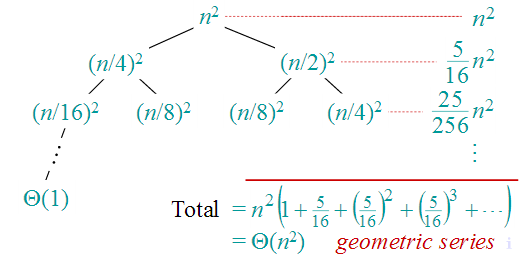
A recursion tree is useful for visualizing what happens when a recurrence is iterated. It diagrams the tree of recursive calls and the amount of work done at each call. For E.g:, Recurrence is T(n) = 2T(n/2) + n². The recursion tree for this recurrence has the following form:

Sum across each row of the tree to obtain the total work done at a given level

This a geometric series, thus in the limit the sum is O(n²)

Q. T(n) = T(n/4) + T(n/2) + n²

“Cookbook” for solving recurrences of the form:

\( T(n) = aT(\frac{n}{b}) + f(n) \)

Where, a ≥ 1; b > 1 and f(n) > 0

Then, depending on the comparison between f(n), \( n^{{log}_b^a} \) there are three cases:

f(n) is asymptotically smaller or larger than \( n^{{log}_b^a} \) by a polynomial factor \( n^{\varepsilon} \)

f(n) is asymptotically equal with \( n^{{log}_b^a} \)

Case 1: f(n) = \( n^{{log}_b^a - \epsilon} \) for some ε > 0 then T(n) = Θ( \( n^{{log}_b^a}) \)

Case 2: f(n) = Θ( \( n^{{log}_b^a}) \) then T(n) = Θ( \( n^{{log}_b^a}) lg n\)

Case 3: f(n) = Ω( \( n^{{log}_b^a + \epsilon} \) ) for some ε > 0 then, and if af(n/b) ≤ cf(n) for some c < 1 and all sufficiently large n, then: T(n) = Θ(f(n))

Q. The time complexity of computing the transitive closure of a binary relation on a set of n elements is known to be (GATE 2005)

O (n)

O (n log n)

O(n³⁄₂)

O(n³)

Ans . (a)

In mathematics, the transitive closure of a binary relation R on a set X is the smallest transitive relation on X that contains R. If the original relation is transitive, the transitive closure will be that same relation; otherwise, the transitive closure will be a different relation.

Q. The recurrence relation capturing the optimal execution time of the Towers of Hanoi problem with n discs is(GATE 2012)

T(n)=2T(n-2)+2

T(n)=2T(n-1)+n

T(n)=2T(n/2)+1

T(n)=2T(n-2)+1

Ans . 4

Let the three pegs be A,B and C respectively. Our goal is to move 'n' pegs from A to C with the help of peg B. The steps to do this are as follows:

move n−1 discs from A to B. This leaves \(n^{th}\) disc alone on peg A --- T(n-1)
move \(n^{th}\) disc from A to C --- 1
move n−1 discs from B to C so they sit on \(n^{th}\) disc --- T(n-1)
By adding the above we get
T(n) = T(n-1) + T(n-1) + 1
i.e T(n)=2T(n-2)+1

upscfever.com

Journey of a Thousand Miles begins with One Click!!!

Divide-and-Conquer

Maximum Subarray Problem

Algorithm for matrix multiplication

Strassen’s Algorithm for matrix multiplication

Solving Recurrance relation - Iteration method

Solving Recurrance relation - Recurrance Tree method

Master's Theorem: Solving Recurrence

UPSCFEVER - POPULAR PAGES

Join The Movement

Discussions and Comments