1. The quicksort algorithm has a worst-case running time of Θ(n²)on an input array of n numbers.




2. Despite this slow worst-case running time, quicksort is often the best practical choice for sorting because it is remarkably efficient on the average: its expected running time is Θ(n lg n), and the constant factors hidden in the Θ(n lg n) notation are quite small.




3. It also has the advantage of sorting in place and it works well even in virtual-memory environments.

1. Quick-sort, like merge sort, applies the divide-and-conquer paradigm . The three-step divide-and-conquer process for sorting a typical subarray A[p ... r]




2. Divide: Partition (rearrange) the array A[p... r] into two (possibly empty) sub-arrays A[p... q-1] and A[q+1 ...r] such that each element of A[p...q - 1] is less than or equal to A[q], which is, in turn, less than or equal to each element of A[q + 1 ... r]. Compute the index q as part of this partitioning procedure.




3. Conquer: Sort the two sub-arrays A[p ... q-1] and A[q+1 ... r] by recursive calls to quick-sort.




4. Combine: Because the subarrays are already sorted, no work is needed to combine them: the entire array A[p...r] is now sorted.

1. QUICKSORT(A,p,r)

2. if p < r

3.     q = PARTITION(A,p,r)

4.     QUICKSORT(A,p,q-1)

5.     QUICKSORT(A,q+1,r)

1. PARTITION(A,p,r)

2. x = A[r]

3. i = p - 1

4. for j = p to r - 1

5.     if A[j] ≤ x

6.        i = i + 1

7.        exchange A[i] with A[j]

8. exchange A[i+1] with A[r]

9. return i + 1

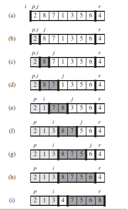
1. The operation of PARTITION on a sample array. Array entry A[r] becomes the pivot element x. Lightly shaded array elements are all in the first partition with values no greater than x. Heavily shaded elements are in the second partition with values greater than x.

2. The unshaded elements have not yet been put in one of the first two partitions, and the final white element is the pivot x.

3. Fig (a) The initial array and variable settings. None of the elements have been placed in either of the first two partitions. Fig(b) The value 2 is “swapped with itself” and put in the partition of smaller values.

4. Fig (c)–(d) The values 8 and 7 are added to the partition of larger values. (e) The values 1 and 8 are swapped, and the smaller partition grows. (f) The values 3 and 7 are swapped, and the smaller partition grows.

5. Fig (g)–(h) The larger partition grows to include 5 and 6, and the loop terminates. Fig (i) In lines 7–8, the pivot element is swapped so that it lies between the two partitions

1. The worst-case behavior for quicksort occurs when the partitioning routine produces one subproblem with n - 1 elements and one with 0 elements.

2. The worst-case running time of quicksort is when the input array is already completely sorted Θ(n²)

3. T(n) = Θ(n lg n) occurs when the PARTITION function produces balanced partition.

4. Sorts in place. If the subarrays are balanced, then quicksort can run as fast as mergesort. If they are unbalanced, then quicksort can run as slowly as insertion sort.





5. Worst-case partitioning: Recurrance Relation

1. T (n) = T (n − 1) + T (0) + Θ(n)

2. = T (n − 1) + Θ(n)

3. = Θ(n²)

6. Best-case partitioning: Recurrance Relation

1. T (n) = 2T (n/2) + Θ(n)

2. = Θ(n lg n)

1. We have assumed that all input permutations are equally likely. This is not always true. To correct this, we add randomization to quicksort.

2. We could randomly permute the input array.

3. Instead, we use random sampling, or picking one element at random.

4. Don't always use A[r] as the pivot. Instead, randomly pick an element from the subarray that is being sorted. We add this randomization by not always using A[r] as the pivot, but instead randomly picking an element from the subarray that is being sorted. Randomly selecting the pivot element will, on average, cause the split of the input array to be reasonably well balanced.

1. RANDOMIZED-PARTITION( A, p, r )

2. i ← RANDOM( p, r )

3. exchange A[r] ↔ A[i]

4. return PARTITION( A, p, r )

1. RANDOMIZED-QUICKSORT( A, p, r )

2. if p < r

3.      then q ← RANDOMIZED-PARTITION( A, p, r )

4.          RANDOMIZED-QUICKSORT( A, p, q − 1)

5.          RANDOMIZED-QUICKSORT( A, q + 1, r)

Quicksort	Mergesort
O(nlogn) is the best case and average case time complexity whereas \(O(n^2)\) is worst case.	The time complexity is independent of the dataset and is O(nlogn) in all cases.
Not a stable sort	Stable sort
Additional space is not required. Superior in terms of space	Extra space is required to store elements during merge.
It has smaller constants in O(nlogn) as compared to merge sort
Quicksort is preferred when the amount of data can fit into main memory. (RAM / internal memory)	For huge amounts of data go for Merge sort
Quick sort is preferred for arrays as lots of restructuring and random access is required as usage of linked list can be expensive	It accesses data sequentially and hence linked lists can be used preferably

1. Counting sort assumes that each of the n input elements is an integer in the range 0 to k, for some integer k. When k = O(n), the sort runs in Θ(n) time.

2. In the code for counting sort, we assume that the input is an array A[1 ... n],and thus A.length = n. We require two other arrays: the array B[1..n] holds the sorted output, and the array C[0...k] provides temporary working storage.

Algorithm of Counting Sort

1. COUNTING-SORT(A,B,k)

2. let C[0...k] be a new array

3. for i = 0 to k

4.     C[i] = 0

5. for j = 1 to A.length

6.     C[A[j]] = C[A[j]] + 1

7. // C[i] now contains the number of elements equal to i.

8. for i = 1 to k

9.    C[i] = C[i] + C[i-1]

10. // C[i] now contains the number of elements less than or equal to i 

11. for j = A.length downto 1

12.    B[C[A[j]]] = A[j]

13.    C[A[j]] = C[A[j]] - 1

Working of Counting Sort

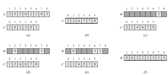
1. The operation of COUNTING-SORT on an input array A[1...8], where each element of A is a nonnegative integer no larger than k = 5. (a) The array A and the auxiliary array C after line 5. (b) The array C after line 8. (c)–(e) The output array B and the auxiliary array C after one, two, and three iterations of the loop in lines 10–12, respectively. Only the lightly shaded elements of array B have been filled in. (f) The final sorted output array B




2. After the for loop of lines 2–3 initializes the array C to all zeros, the for loop of lines 4–5 inspects each input element. If the value of an input element is i , we increment C[i]. Thus, after line 5, C[i] holds the number of input elements equal to i for each integer i = {0; 1; ...; k}. Lines 7–8 determine for each i = {0; 1; ...; k} how many input elements are less than or equal to i by keeping a running sum of the array C.




3. Finally, the for loop of lines 10–12 places each element A[j] into its correct sorted position in the output array B.If all n elements are distinct, then when we first enter line 10, for each A[j] ,the value C[A[j]] is the correct final position of A[j] in the output array, since there are C[A[j]] elements less than or equal to A[j].




4. Because the elements might not be distinct, we decrement C[A[j]] each time we place a value A[j] into the B array. Decrementing C[A[j]] causes the next input element with a value equal to A[j], if one exists, to go to the position immediately before A[j] in the output array.

Runtime of Counting Sort

1. The Ω(n lg n) is the lower bound for sorting of category of comparison sort.

2. An important property of counting sort is that it is stable so numbers with the same value appear in the output array in the same order as they do in the input array.

3. Runtime is Θ(n)

Exercises of Counting Sort

Q. illustrate the operation of COUNTING-SORT on the array A = {6; 0; 2; 0; 1; 3; 4; 6; 1; 3; 2}.

1. We have that C = {2; 4; 6; 8; 9; 9; 11}. Then, after successive iterations of the loop on lines 10-12, we have B = {; ; ; ; ; 2; ; ; ; ; } B = { ; ; ; ; ; 2; ; 3; ; ; } ,B = { ; ; ; 1; ; 2; ; 3; ; ; } and at the end, B = {0; 0; 1; 1; 2; 2; 3; 3; 4; 6; 6}

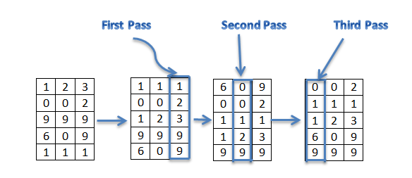
1. Radix sort solves the problem of card sorting counter intuitively by sorting on the least significant digit first.




2. The algorithm then combines the cards into a single deck, with the cards in the 0 bin preceding the cards in the 1 bin preceding the cards in the 2 bin, and so on.




3. Then it sorts the entire deck again on the second-least significant digit and recombines the deck in a like manner. The process continues until the cards have been sorted on all d digits. Remarkably, at that point the cards are fully sorted on the d-digit number. Thus, only d passes through the deck are required to sort.

Example of Radix Sort

1. Original, unsorted list: 170, 45, 75, 90, 802, 2, 24, 66

2. Sorting by least significant digit (1s place) gives: 170, 90, 802, 2, 24, 45, 75, 66. Notice that we keep 802 before 2, because 802 occurred before 2 in the original list, and similarly for pairs 170 & 90 and 45 & 75

3. Sorting by next digit (10s place) gives: 802, 2, 24, 45, 66, 170, 75, 90 Notice that 802 again comes before 2 as 802 comes before 2 in the previous list.

4. Sorting by most significant digit (100s place) gives: 2, 24, 45, 66, 75, 90, 170, 802. It is important to realize that each of the above steps requires just a single pass over the data, since each item can be placed in its correct bucket without having to be compared with other items.

1. RADIX-SORT(A,d)

2. for i = 1 to d

3.     use a stable sort to sort array A on digit i

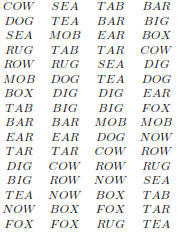
Q. illustrate the operation of RADIX-SORT on the following list of English words: COW, DOG, SEA, RUG, ROW, MOB, BOX, TAB, BAR, EAR, TAR, DIG, BIG, TEA, NOW, FOX.

1. Starting with the unsorted words on the left, and stable sorting by progressively more important positions.

1. BUCKET-SORT(A)

2. let B[0...n-1] be a new array

3. n = A.length

4. for i = 0 to n - 1

5.     make B[i] an empty list

6. for i = 1 to n

7.     insert A[i] into list B[nA[i]]

8. for i = 0 to n - 1

9.     sort list B[i] with insertion sort

10. concatenate the lists B[0]; B[1]; : : : ; B[n-1] together in order

Average-case running time for bucket sort is Θ(n)

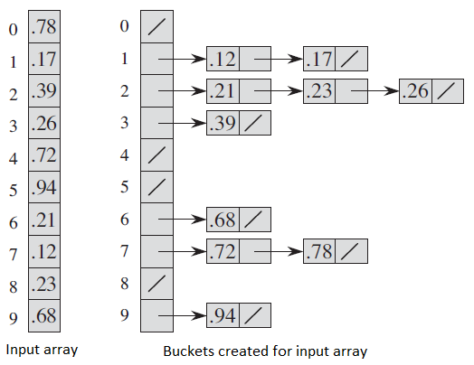
1. The operation of BUCKET-SORT for n = 10. (a) The input array A[1...10]. (b) The array B[0...9] of sorted lists (buckets) after line 8 of the algorithm.




2. Bucket i holds values in the half-open interval [i/10, (i + 1)/10).




3. The sorted output consists of a concatenation in order of the lists B[0]; B[1]; .... ; B[9].

Q.1 Which one of the following is the recurrence equation for the worst case time complexity of the Quicksort algorithm for sorting (n > = 2) numbers? In the recurrence equations given in the options below, c is a constant.(Gate 2015 Set1)

1. T(n) = 2T(n=2) + cn




2. T(n) = T(n – 1) + T(0) + cn




3. T(n) = 2T(n – 2) + cn




4. T(n) = T(n=2) + cn

Ans: (B)

1. In worst case, the chosen pivot is always placed at a corner position and recursive call is made for following. a) for subarray on left of pivot which is of size n-1 in worst case. b) for subarray on right of pivot which is of size 0 in worst case.

Q. A max-heap is a heap where the value of each parent is greater than or equal to the value of its children. Which of the following is a max-heap? (GATE 2011)

1. 




2. 




3. 




4. 

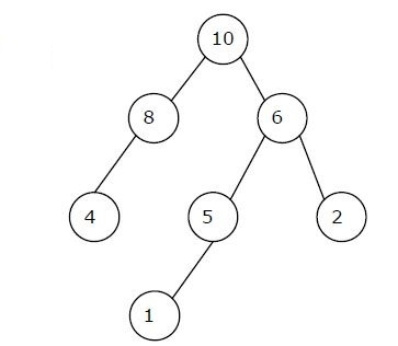
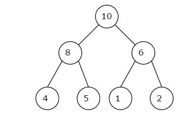
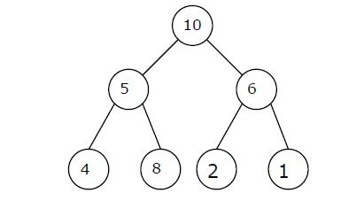
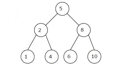
Ans . 2

1. Heap is a complete binary tree

Q. In quick sort, for sorting n elements, the $(n/4)th$ the smallest element is selected as pivot using an O(n) time algorithm. What is the worst case time complexity of the quick sort? (GATE 2009)

(A)Θ(n)
(B) Θ(nlogn)
(C)Θ(n^2)
(D)Θ(n^2logn)

Ans . B

The recursion expression becomes:
T(n) = T(n/4) + T(3n/4) + cn
which is the average case complexity. And average case complexity of quick sort is θ(nlogn)

Q. Consider the Quicksort algorithm. Suppose there is a procedure for finding a pivot element which splits the list into two sub-lists each of which contains at least one-fifth of the elements. Let T(n) be the number of comparisons required to sort n elements. Then (GATE Paper-2008)

1. T(n) <= 2T(n/5) + n




2. T(n) <= T(n/5) + T(4n/5) + n




3. T(n) <= 2T(4n/5) + n




4. T(n) <= 2T(n/2) + n

Ans . (3)

Explanation :

For the case where n/5 elements are in one subset, T(n/5) comparisons are needed for the first subset with n/5 elements, T(4n/5) is for the rest 4n/5 elements, and n is for finding the pivot. If there are more than n/5 elements in one set then other set will have less than 4n/5 elements and time complexity will be less than T(n/5) + T(4n/5) + n because recursion tree will be more balanced.

Q.1 You have an array of n elements. Suppose you implement quicksort by always choosing the central element of the array as the pivot. Then the tightest upper bound for the worst case performance is (GATE 2014 SET 3)

1. \( O{(n)^2} \)


2. \(O(n\log n)\)


3. \(\theta (n\log n)\)



4. \(O{\left( n \right)^3}\)

Ans . \( O{\left( n \right)^2}\)

1. The central element may always be an extreme element, therefore time complexity in worst case becomes \(O{\left( n \right)^2}\)

(SET April 2017 Paper-II A)

Q. Merging 4 sorted files containing 50, 10, 25 and 15 records will take ______ time

1. (A) O(100)




2. (B) O(200)




3. (C) O(175)




4. (D) O(125)

Ans. (A) O(100)

Explanation:

1. Time Complexity of Merge sort is O(n log n). But Combine step or Merging a total of 'n' elements taking O(n) time. So, O(100) is the correct option here as total 100 records to merged.

(SET April 2017 Paper-III A)

Q. For sorting ______ algorithm scans the list by swapping the entries whenever pair of adjacent keys are out of desired order.

1. (A) Quick sort




2. (B) Shell sort




3. (C) Insertion sort




4. (D) Bubble Sort

Ans. (D) Bubble Sort

Explanation:

1. As in bubble sort always we swap the adjacent keys if they are not in desired order.

Q. For the following:

1. To solve a problem linear algorithm must perform faster than quadratic algorithm




2. An algorithm with worst case time behavior = 3n takes 30 operations for every input of size n=10

1. (A) Both (i) and (ii) are false




2. (B) Both (i) and (ii) are true




3. (C) (i) is false and (ii) is true




4. (D) (i) is true and (ii) is false

Ans. (D) (i) is true and (ii) is false

Explanation:

1. As the first statement is true according to the definition of linear algorithms, the second is false as 30 operations are not needed.

Q. The best/worst case time complexity of quick sort is:

1. (A) O(n)/O(n²)




2. (B) O(n)/O(n log n)




3. (C) O(n log n)/O(n²)




4. (D) O(n log n)/O(n log n)

Ans. (C) O(n log n)/O(n²)

Explanation:

1. For quick sort best case time complexity is O(n log n) & worst case time complexity is O(n²).

Q 5. What is the number of swaps required to sort n elements using selection sort, in the worst case?(GATE 2009)

1. θ(n)




2. θ(n Log n)




3. θ(n*n)




4. θ(n*nLog n)

Ans: A

Q 6.In quick sort, for sorting n elements, the (n/4)th smallest element is selected as pivot using an O(n) time algorithm. What is the worst case time complexity of the quick sort? (GATE 2009)

1. θ(n)




2. θ(n Log n)




3. θ(n*n)




4. θ(n*nLog n)

Ans: B

Q 7.

I.  There exist parsing algorithms for some programming languages 
     whose complexities are less than O(n3).
II.  A programming language which allows recursion can be implemented 
    with static storage allocation.
III. No L-attributed definition can be evaluated in The framework 
     of bottom-up parsing.
IV. Code improving transformations can be performed at both source 
    language and intermediate code level.

(GATE 2009)

1. I and II




2. I and IV




3. III and IV




4. I,III and IV

Ans: B

Previous

Next