Scheduling Algorithms - First-Come, First-Served Scheduling
CPU scheduling deals with the problem of deciding which of the processes in the ready queue is to be allocated the CPU.
In FCFS the process that requests the CPU first is allocated the CPU first.
The implementation of the FCFS policy is easily managed with a FIFO queue. When a process enters the ready queue, its PCB is linked onto the tail of the queue.
When the CPU is free, it is allocated to the process at the head of the queue. The running process is then removed from the queue.
On the negative side, the average waiting time under the FCFS policy is often quite long.
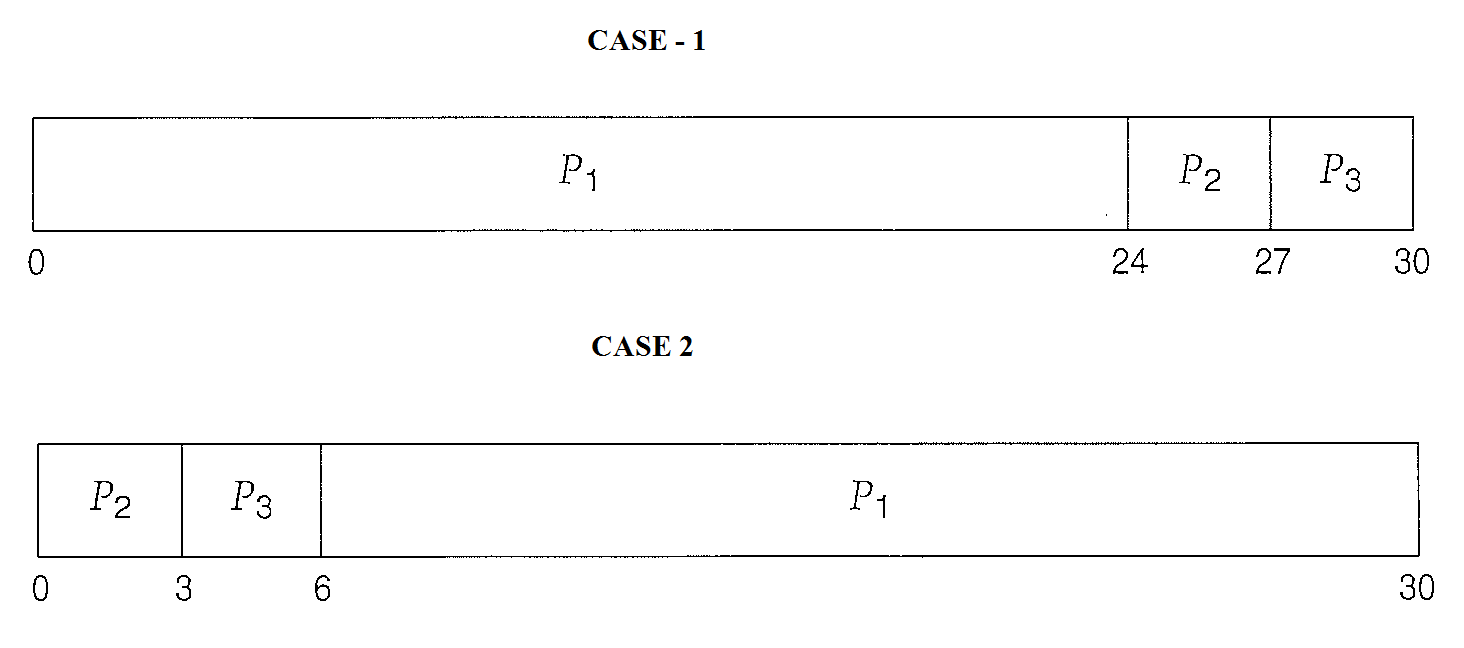
Q. Consider the process and their burst times as given in the table
| Process | Burst time |
|---|---|
| P1 | 24 |
| P2 | 3 |
| P3 | 3 |
The processes arrive in the order of P1, P2 and P3 then we get the following order
The waiting time for P1 is 0 ms, P2 is 24 and P3 is 27 ms. Thus, the average waiting time is (0 + 24 + 27)/3 = 17 ms.
But if the processes arrive in the order P2, P3 and P1 then the average waiting time is now (6 + 0 + 3)/3 = 3 msmilliseconds. This reduction is substantial. Thus, the average waiting time under an FCFS policy is generally not minimal and may vary substantially if the processes CPU burst times vary greatly.
There is a convoy effect possible in FCFS if the other small CPU burst processes wait for the one big process to get off the CPU. This effect results in lower CPU and device utilization than might be possible if the shorter processes were allowed to go first.
FCFS scheduling algorithm is non-preemptive. Once the CPU has been allocated to a process, that process keeps the CPU until it releases the CPU, either by terminating or by requesting I/0. The FCFS algorithm is thus particularly troublesome for time-sharing systems, where it is important that each user get a share of the CPU at regular intervals.
Shortest-Job-First Scheduling (shortest-next-CPU-burst algorithm)
This algorithm associates with each process the length of the process's next CPU burst.
When the CPU is available, it is assigned to the process that has the smallest next CPU burst.
If the next CPU bursts of two processes are the same, FCFS scheduling is used to break the tie.
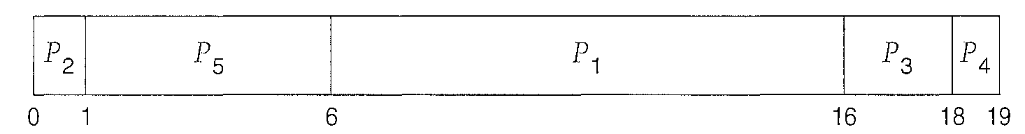
Consider the following set of processes, with the length of the CPU burst given in milliseconds:
The waiting time is 3 milliseconds for process P 1 , 16 milliseconds for process P 2 , 9 milliseconds for process P 3 , and 0 milliseconds for process P 4 . Thus, the average waiting time is (3 + 16 + 9 + 0) / 4 = 7 milliseconds.
By comparison, if we were using the FCFS scheduling scheme, the average waiting time would be 10.25 milliseconds.
The SJF scheduling algorithm is provably optimal, in that it gives the minimum average waiting time for a given set of processes.
Moving a short process before a long one decreases the waiting time of the short process more than it increases the waiting time of the long process. Consequently, the average waiting time decreases.
SJF scheduling is used frequently in long-term scheduling.
Although the SJF algorithm is optimal, it cannot be implemented at the level of short-term CPU scheduling. With short-term scheduling, there is no way to know the length of the next CPU burst.
The SJF algorithm can be either preemptive or nonpreemptive.
A preemptive SJF algorithm will preempt the currently executing process, whereas a nonpreemptive SJF algorithm will allow the currently running process to finish its CPU burst. Preemptive SJF scheduling is sometimes called shortest-remaining-time-first scheduling.
| Process | Burst time |
|---|---|
| P1 | 6 |
| P2 | 8 |
| P3 | 7 |
| P3 | 3 |
Q. Consider the process and their burst times as given in the table
| Process | Arrival time | Burst time |
|---|---|---|
| P1 | 0 | 8 |
| P2 | 1 | 4 |
| P3 | 2 | 9 |
| P4 | 3 | 5 |
Process P 1 is started at time 0, since it is the only process in the queue. Process P 2 arrives at time 1. The remaining time for process P 1 (7 milliseconds) is larger than the time required by process P 2 (4 milliseconds), so process P 1 is preempted, and process P 2 is scheduled.
The average waiting time for this example is [(10- 1) + (1 - 1) + (17- 2) +(5-3)]/ 4 = 26/4 = 6.5 milliseconds.
Nonpreemptive SJF scheduling would result in an average waiting time of 7.75 milliseconds.
Priority Scheduling
The SJF algorithm is a special case of the general priority scheduling algorithm. A priority is associated with each process, and the CPU is allocated to the process with the highest priority.
Equal-priority processes are scheduled in FCFS order.
An SJF algorithm is simply a priority algorithm where the priority (p) is the inverse of the (predicted) next CPU burst.
The larger the CPU burst, the lower the priority, and vice versa.
Priorities can be defined either internally or externally. Internally defined priorities use some measurable quantity or quantities to compute the priority of a process.
External priorities are set by criteria outside the operating system, such as the importance of the process etc.
Priority scheduling can be either preemptive or non-preemptive. When a process arrives at the ready queue, its priority is compared with the priority of the currently running process.
A preemptive priority scheduling algorithm will preempt the CPU if the priority of the newly arrived process is higher than the priority of the currently running process.
A non preemptive priority scheduling algorithm will simply put the new process at the head of the ready queue.
A major problem with priority scheduling algorithms is indefinite blocking, or starvation. A priority scheduling algorithm can leave some low priority processes waiting indefinitely.
A solution to the problem of indefinite blockage of low-priority processes is aging. Aging is a technique of gradually increasing the priority of processes that wait in the system for a long time.
Q. Using priority scheduling, we would schedule these processes according to the following Gantt chart:
| Process | Arrival time | Burst time |
|---|---|---|
| P1 | 10 | 3 |
| P2 | 1 | 1 |
| P3 | 2 | 4 |
| P4 | 1 | 5 |
| P5 | 5 | 2 |
The average waiting time is 8.2 milliseconds.
Round-Robin Scheduling
The round-robin (RR) scheduling algorithm is designed especially for time sharing systems. It is similar to FCFS scheduling, but preemption is added to enable the system to switch between processes.
A small unit of time, called a time quantum or time slice, is defined.
A time quantum is generally from 10 to 100 milliseconds in length. The ready queue is treated as a circular queue.
The CPU scheduler goes around the ready queue, allocating the CPU to each process for a time interval of up to 1 time quantum.
The average waiting time under the RR policy is often long.
In the RR scheduling algorithm, no process is allocated the CPU for more than 1 time quantum in a row (unless it is the only runnable process).
If a process's CPU burst exceeds 1 time quantum, that process is preempted and is put back in the ready queue. The RR scheduling algorithm is thus preemptive.
At one extreme, if the time quantum is extremely large, the RR policy is the same as the FCFS policy.
In contrast, if the time quantum is extremely small (say, 1 millisecond), the RR approach is called processor sharing and (in theory) creates the appearance that each of the "n" processes has its own processor running at 1/nth the speed of the real processor.
Although the time quantum should be large compared with the context switch time, it should not be too large. If the time quantum is too large, RR scheduling degenerates to an FCFS policy. A rule of thumb is that 80 percent of the CPU bursts should be shorter than the time quantum.
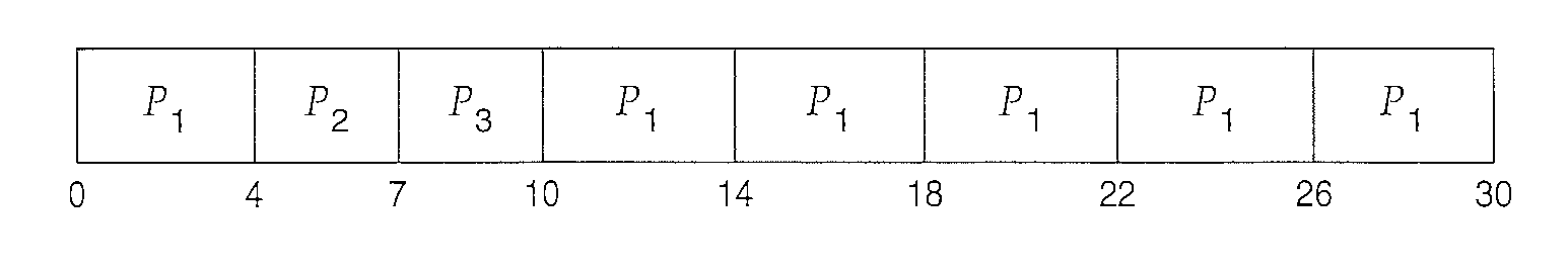
Q. Apply RR scheduling on the below processes (quantum = 4ms)
| Process | Arrival time | Burst time |
|---|---|---|
| P1 | 24 | |
| P2 | 3 | |
| P3 | 3 |
If we use a time quantum of 4 milliseconds, then process P 1 gets the first 4 milliseconds. Since it requires another 20 milliseconds, it is preempted after the first time quantum, and the CPU is given to the next process in the queue, process P 2 .
Process P 2 does not need 4 milliseconds, so it quits before its time quantum expires. The CPU is then given to the next process, process P3. Once each process has received 1 time quantum, the CPU is returned to process P 1 for an additional time quantum.
The resulting RR schedule is as follows:
Thus, the average waiting time is 17/3 = 5.66 milliseconds.