Dynamic programming
Dynamic programming, like the divide-and-conquer method, solves problems by combining the solutions to subproblems.
Dynamic programming applies when the subproblems overlap—that is, when subproblems share subsubproblems. In this context, a divide-and-conquer algorithm does more work than necessary, repeatedly solving the common subsubproblems.
A dynamic-programming algorithm solves each subsubproblem just once and then saves its answer in a table, thereby avoiding the work of recomputing the answer every time it solves each subsubproblem.
When developing a dynamic-programming algorithm, we follow a sequence of four steps:
Characterize the structure of an optimal solution.
Recursively define the value of an optimal solution.
Compute the value of an optimal solution, typically in a bottom-up fashion.
Construct an optimal solution from computed information.
There are usually two equivalent ways to implement a dynamic-programming approach.
The first approach is top-down with memoization. In this approach, we write the procedure recursively in a natural manner, but modified to save the result of each subproblem (usually in an array or hash table). The procedure now first checks to see whether it has previously solved this subproblem. If so, it returns the saved value, saving further computation at this level; if not, the procedure computes the value in the usual manner. We say that the recursive procedure has been memoized; it “remembers” what results it has computed previously.
The second approach is the bottom-up method. This approach typically depends on some natural notion of the “size” of a subproblem, such that solving any particular subproblem depends only on solving “smaller” subproblems. We sort the subproblems by size and solve them in size order, smallest first. When solving a particular subproblem, we have already solved all of the smaller subproblems its solution depends upon, and we have saved their solutions. We solve each subproblem only once, and when we first see it, we have already solved all of its prerequisite subproblems.
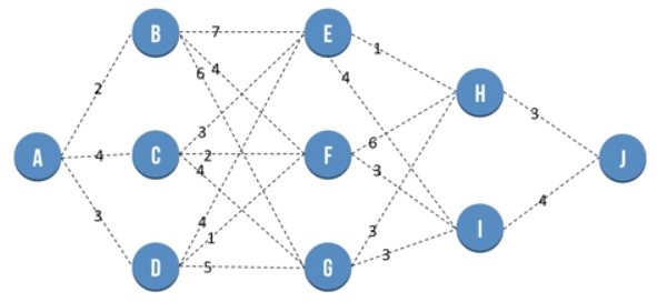
Dynamic programming - Principle of Optimality
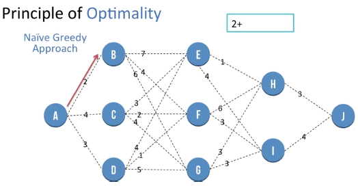
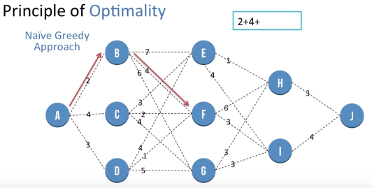
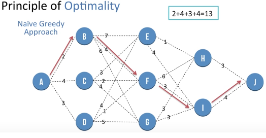
Let the Goal be to reach from Source (Node A) to Destination (Node J). We first use the Naive greedy approach of choosing the local optimal solution at every stage.
Hence we first go from A to B
Then we go from B to F
Then we go from F to I
Then we go from I to J, the path cost use 13 units. But there exist another path which is shorter and the greedy approach wont find it so we need another approach known as "Dynamic programming".
Dynamic Programming - Principle of Optimality
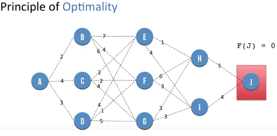
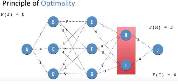
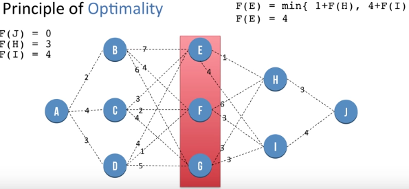
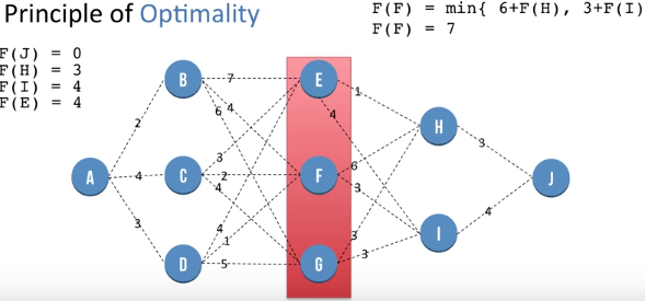
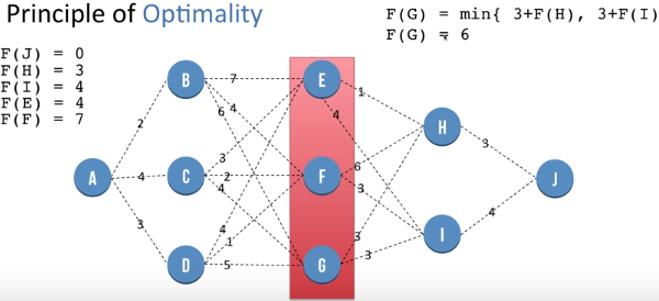
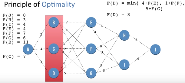
Let F(X) be the minimum distance needed to go to J from node X. F(J) is the distance of going from J to J and so is 0.
F(H) = 3 and F(I) = 4. By the similar method as above.
F(E) = min {1 + F(H) , 4 + F(I) }. This helps us reach a global optimal value at node E by using previously saved information about nodes H and I. So we get F(E) = 4 . Similarly we repea process for nodes at same level of E i.e F and G and we get F(F) = 7 and F(G) = 6. We store these values for further use.
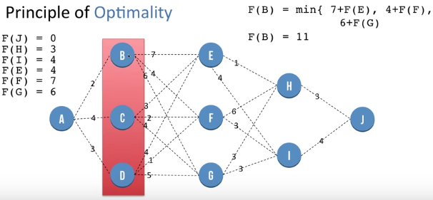
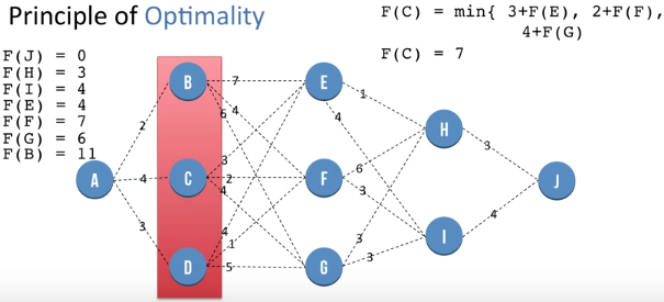
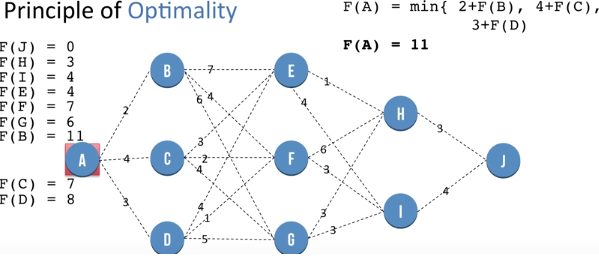
We repea the same procedure to get value of F(B), F(C) and F(D) which is at 11, 7 and 8 respectively.
Finally we get the value of F(A) as 11 which is better than the greedy approach.
Matrix Chain Multiplication
Matrix multiplication is associative, and so all parenthesizations yield the same product. if the chain of matrices is \( A_1, A_2, A_3, A_4 \) i, then we can fully parenthesize the product \( A_1 . A_2 . A_3 . A_4 \) in five distinct ways: \( (A_1 .( A_2 . (A_3 . A_4))) \) , \( (A_1 .(( A_2 . (A_3 ). A_4)) \), \( ((A_1 . A_2 ). (A_3 . A_4)) \) and so on
If A is a p * q matrix and B is a q * r matrix, the resulting matrix C is a p * r matrix. The time to compute C is dominated by the number of scalar multiplications which is pqr
Matrix Chain Multiplication - Pseudocode
MATRIX-CHAIN-ORDER(p)
n = p.length - 1
let m[1..n, 1..n] and s[1..n-1, 2..n] be new tables
for i = 1 to n
m[i,i] = 0
for l = 2 to n
for i = 1 to n - l + 1
j = i + l - 1
m[i,j] = ∞
for k = i to j - 1
q = m[i,k] + m[k+1, j] + pi-1*pk*pj
if q < m[i,j]
m[i,j] = q
s[i,j] = k
return m and s
Matrix Chain Multiplication - Operation
Example Showing Tables and Calculations
- Array dimensions:
- A1: 2 x 3
- A2: 3 x 5
- A3: 5 x 2
- A4: 2 x 4
- A5: 4 x 3
- Tables of \(M_{ij} \) and \(d_j \):
- Initially all M[i,i] = 0, so M[1,1] = M[2,2] = M[3,3] = M[4,4] = M[5,5] = 0.
- M[1,2] = M[1,1] + M[2,2] + \( P_0 * P_2 * P_1 \)
- M[2,3] = M[2,2] + M[3,3] + \( P_1 * P_2 * P_3 \)
- M[3,4] = M[3,3] + M[4,4] + \( P_2 * P_3 * P_4 \)
- M[4,5] = M[4,4] + M[5,5] + \( P_3 * P_4 * P_5 \)
- M[1,5] = M[4,4] + M[5,5] + \( P_3 * P_4 * P_5 \)
- Calculating \(M_{3,5} \) =
- Calculating \(M_{1,3} \) =
- Calculating \(M_{2,4} \) =
- Calculating \(M_{1,4} \) =
- Calculating \(M_{25} \) = number of multiplies in the optimal way to parenthesize \(A_2A_3A_4A_5 \):
- Optimal locations for parentheses: \( \begin{array}{c|ccccc} i,j & 1 & 2 & 3 & 4 & 5 \\ \hline 1 & & 1 & 1 & 3 & 3 \\ 2 & & & 2 & 3 & \color{orange}{3} \\ 3 & & & & 3 & 3 \\ 4 & & & & & 4 \\ 5 & & & & & \end{array} \)
Array sizes: Ai = di-1 by di : \( \begin{array}{c|ccccc} j & 0 & 1 & 2 & 3& 4 & 5 \\ \hline d_j & 2 & \color{magenta}{3} & \color{blue}{5} & \color{orange}{2} & \color{red}{4} & \color{magenta}{3} \end{array} \) This is the input parameter 'p' passed to the function.
Mij = number of multiplies in best way to parenthesize arrays Ai .. Aj: \( \begin{array}{c|ccccc} i,j & 1 & 2 & 3 & 4 & 5 \\ \hline 1 & 0 & 30 & 42 & 58 & 78 \\ 2 & & \color{blue}{0} & \color{orange}{30} & \color{red}{ 54} & \color{cyan}{72} \\ 3 & & & 0 & 40 & \color{blue} {54} \\ 4 & & & & 0 &\color{orange}{24} \\ 5 & & & & &\color{red }{0} \end{array} \)
\( \color{cyan}{M_{3,5}} = \min \begin{cases} \color{blue }{M_{33} + M_{45}} + \color{magenta}{p_2}\color{blue }{p_3}\color{magenta}{p_5}, \\ \color{orange}{M_{34} + M_{55}} +\color{magenta}{p_2}\color{orange}{p_4}\color{magenta}{p_5} \end{cases} \)
\( \color{cyan}{M_{1,3}} = \min \begin{cases} \color{blue }{M_{11} + M_{23}} + \color{magenta}{p_0}\color{blue }{p_3}\color{magenta}{p_1}, \\ \color{orange}{M_{12} + M_{33}} +\color{magenta}{p_0}\color{orange}{p_3}\color{magenta}{p_2} \end{cases} \)
\( \color{cyan}{M_{2,4}} = \min \begin{cases} \color{blue }{M_{22} + M_{34}} + \color{magenta}{p_1}\color{blue }{p_4}\color{magenta}{p_2}, \\ \color{orange}{M_{23} + M_{44}} +\color{magenta}{p_1}\color{orange}{p_3}\color{magenta}{p_4} \end{cases} \)
\( \color{cyan}{M_{1,4}} = \min \begin{cases} \color{blue }{M_{11} + M_{24}} + \color{magenta}{p_0}\color{blue }{p_1}\color{magenta}{p_4}, \\ \color{orange}{M_{12} + M_{34}} +\color{magenta}{p_0}\color{orange}{p_2}\color{magenta}{p_4}, \\ \color{orange}{M_{13} + M_{44}} +\color{magenta}{p_0}\color{orange}{p_3}\color{magenta}{p_4} \\ \end{cases} \)
\( \color{cyan}{M_{25}} = \min \begin{cases} \color{blue }{M_{22} + M_{35}} + \color{magenta}{d_1}\color{blue }{d_2}\color{magenta}{d_5}, \\ \color{orange}{M_{23} + M_{45}} +\color{magenta}{d_1}\color{orange}{d_3}\color{magenta}{d_5}, \\ \color{red}{M_{24} + M_{55}} + \color{magenta}{d_1}\color{red}{d_4}\color{magenta}{d_5} \end{cases} \) \( = \min \begin{cases} 0 + 54 + 45 = 99 \\ 30 + 24 + 18 = 72 \\ 54 + 0 + 36 = 90 \end{cases} \) \( = \min \begin{cases} (A_2)(A_3A_4A_5)\\ (A_2A_3)(A_4A_5)\\ (A_2A_3A_4)(A_5) \end{cases} \)
\( A_1 . A_2 . A_3 . A_4 . A_5 \) This is the original order and we need to decide where to add the paranthesis. This is done with the help of the second table that is shown above.
Checking entry S[1,5] we obtain 3. This means that \( (A_1 . A_2 . A_3) . (A_4 . A_5) \) as 3 is the first point of parenthesis.
Then we check S[1,3] to obtain second division point as 1 so we have
\( ((A_1) . (A_2 . A_3)) . (A_4 . A_5) \)
Longest Common Sub-sequence
Given two sequences X and Y , we say that a sequence Z is a common subsequence of X and Y if Z is a subsequence of both X and Y . For example, if X = {A; B; C; B; D; A; B} and Y = {B; D; C; A; B; A} the sequence {B; C; A} is a common subsequence of both X and Y .
The sequence {B; C; A} is not a longest common subsequence (LCS) of X and Y , however, since it has length 3 and the sequence {B; C; B; A}, which is also common to both X and Y , has length 4.
The sequence {B; C; B; A} is an LCS of X and Y , as is the sequence {B; D; A; B}, since X and Y have no common subsequence of length 5 or greater.
In a brute-force approach to solving the LCS problem, we would enumerate all subsequences of X and check each subsequence to see whether it is also a subsequence of Y , keeping track of the longest subsequence we find.
Each subsequence of X corresponds to a subset of the indices {1; 2; ... ;m} of X. Because X has 2 subsequences, this approach requires exponential time, making it impractical for long sequences.
Longest Common Sub-sequence - Algorithm
LCS-LENGTH(X,Y)
m = X.length
n = Y.length
let b[1 ... m , 1 .. n] and c[0 ... m , 0 .. n] be new tables
for i = 1 to m
c[i,0] =0
for j = 1 to m
c[j,0] =0
for i = 1 to m
for j = 1 to n
if xi = yi
c[i,j] = c[i-1,j-1] + 1
b[i,j] = "\"
elseif c[i-1,j] ≥ c[i,j-1]
c[i,j] = c[i-1,j]
b[i,j] = "|"
else
c[i,j] = c[i,j-1]
b[i,j] = "<-"
return c and b
PRINT-LCS(b,X,i,j)
if i == 0 and j == 0
return
if b[i,j] == "\"
PRINT-LCS(b,X,i - 1,j - 1)
print xi
elseif b[i,j] == "|"
PRINT-LCS(b,X,i - 1,j)
else PRINT-LCS(b,X,i,j - 1)
Runtime of the procedure LCS-LENGTH(X,Y) is Θ(mn) and of PRINT-LCS(b,X,i,j) is O(m+n). where m and n are lengths of the two strings.
Longest Common Sub-sequence - Example
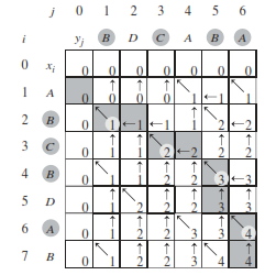
Write anyone of the strings on the x axis and the other string on the y axis as shown above. Then assuming that the matrix is named X , all fields having i=0 or j=0 or both should be initialised to 0. Thus for all X[0,j] and X[i,0] we have X[i,j]=0.
Then for a cell say X[1,1] check the corresponding alphabets of the strings. In this case they are 'A' and 'B'. Since we have both different we get the "elseif" case on the Algorithm of LCS-LENGTH(X,Y) which is line 14. So we put value X[1,1] = 0 as X[0,1] = 0 and the arrow "|" in the cell. Then we move to the next cell in the row i.e X[1,2].
When we reach cell X[1,4] we have corresponding alphabets same as both are 'A' so we reach the line 11 of LCS-LENGTH(X,Y) and X[1,4] = 1 with diagonal arrow.
Continuing in this manner, the rightmost bottom cell of the matrix 'X' indicates the length of the longest common subsequence.
PRINT-LCS(b,X,i,j) working
We start from the right most bottom cell of the matrix given to us i.e. X[7,6]. Since it has the arrow upwards we move from that cell to upward cell i.e. X[6,6].
X[6,6] has the diagonal arrow and whenever we get diagonal arrow we print corresponding character on any axis (since both are same) which in this case is "A".
We continue to follow the path of the arrows and continue to move in direction and print everytime we reach a diagonal arrow. Finally we get the cell X[1,0] and we stop.
Till this time we have the words "A", "B", "C", "B" and the longest common subsequence is obtained by reading this list backward to get "BCAB".
Solved Question Papers
Q. 3 The Floyd-Warshall algorithm for all-pair shortest paths computation is based on (GATE 2016 SET B)
Greedy paradigm.
Divide-and-Conquer paradigm.
Dynamic Programming paradigm.
Neither Greedy nor Divide-and-Conquer nor Dynamic Programming paradigm.
Ans . C
Solution steps: Floyd - warshall algorithm follows dynamic programming paradigm.
Q. Suppose P, Q, R, S, T are sorted sequences having lengths 20, 24, 30,
35, 50 respectively. They are to be merged into a single sequence by merging
together two sequences at a time. The number of comparisons that will be
needed in the worst case by the optimal algorithm for doing this is .
(GATE 2014 SET 2)
Ans . 358
solution
To merge two arrays m+n-1 comparisons are made in worst case where m and n are size of array respectively. For algorithm to optimal smallest arrays must be merged first.
So first merge arrays P and Q will give array of size 44(PQ) in 43 comparisons. Next merging arrays R and S gives array of size 65(RS) in 64 comparison. Next merging PQ and T gives array of size 94(PQT) in 93 comparisons Now merging PQT and RS gives array of size 159 in 158 comparisons. So total comparisons made 43+64+93+158 = 358
Q. Consider two strings A = ”qpqrr” and B = ”pqprqrp”. Let x be the length
of the longest common subsequence (not necessarily contiguous) between A and
B and let y be the number of such longest common subsequences between A
and B. Then x + 10y =___ .
(GATE 2014 SET 2)
Ans . 34
LCS for string A and B is of length 4 therefore length of longest common subsequence is 4 (x = 4).
There are three such subsequences ”qprr”,”pqrr”and ”qpqr”(y = 3).
x = 4 and y = 3.
x+10y = 34
Common data question A subsequence of a given sequence is just the given sequence with some elements (possibly none or all) left out. We are given two sequences X[m] and Y[n] of lengths m and n, respectively, with indexes of X and Y starting from 0. (GATE 2009) Q. We wish to find the length of the longest common subsequence (LCS) of X[m] and Y[n] as l(m, n), where an incomplete recursive definition for the function l(i, j) to compute the length of the LCS of X[m] and Y[n] is given below: l(i, j) = 0, if either i = 0 or j = 0 = expr1, if i, j>0 and x[i ] = [j ] = expr2, if i, j>0 and x[i ] [j ] Which one of the following option is correct?
(A) expr ≡ l(i-1 , j) +1
(B) expr ≡ l(i, j-1)
(C) expr ≡ max(l(i-1,j),1(i,j-1))
(D) expr ≡ max(l(i-1,j-1),1(i,j))
Ans . C
In Longest common subsequence problem, there are two cases for X[0 to i] and Y[0 to j] 1) The last characters of two strings match. The length of lcs is length of lcs of X[0 to i-1] and Y[0 to j-1] 2) The last characters don't match. The length of lcs is max of following two lcs values a) LCS of X[0 to i-1] and Y[0 to j] b) LCS of X[0 to i] and Y[0 to j-1]
Q.1 An algorithm to find the length of the longest monotonically increasing sequence of numbers in an array A [0 - n-1] is given below.
Let Li denote the length of the longest monotonically increasing sequence starting at index i in the array for all such that 0 <= i <= n-2
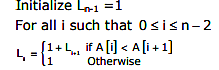 Finally the length of the longest monotonically increasing sequence is Max(L0,L1,....,Ln-1)
Which of the following statements is TRUE?
(GATE 2011)
Finally the length of the longest monotonically increasing sequence is Max(L0,L1,....,Ln-1)
Which of the following statements is TRUE?
(GATE 2011)
The algorithm uses dynamic programming paradigm
The algorithm has a linear complexity and uses branch and bound paradigm
The algorithm has a non-linear polynomial complexity and uses branch and bound paradigm
The algorithm uses divide and conquer paradigm
Ans . (A)