The area of the region bounded by the curve y = f (x), x-axis and the lines x = a and x = b (b > a) is given by the formula:

The area of the region bounded by the curve x = φ (y), y-axis and the lines y = c, y = d is given by the formula:

The area of the region enclosed between two curves y = f (x), y = g (x) and the lines x = a, x = b is given by the formula,

If f (x) ≥ g (x) in [a, c] and f (x) ≤ g (x) in [c, b], a < c < b, then

An equation involving derivatives of the dependent variable with respect to independent variable (variables) is known as a differential equation.

Order of a differential equation is the order of the highest order derivative occurring in the differential equation.

Degree of a differential equation is defined if it is a polynomial equation in its derivatives.

Degree (when defined) of a differential equation is the highest power (positive integer only) of the highest order derivative in it.

A function which satisfies the given differential equation is called its solution. The solution which contains as many arbitrary constants as the order of the differential equation is called a general solution and the solution free from arbitrary constants is called particular solution

To form a differential equation from a given function we differentiate the function successively as many times as the number of arbitrary constants in the given function and then eliminate the arbitrary constants.

Variable separable method is used to solve such an equation in which variables can be separated completely i.e. terms containing y should remain with dy and terms containing x should remain with dx.

A differential equation which can be expressed in the form $\frac{dy}{dx} = f(x,y)$ or $\frac{dx}{dy} = g(x,y)$ where, f (x, y) and g(x, y) are homogenous functions of degree zero is called a homogeneous differential equation

A differential equation of the form $\frac{dy}{dx} + Py = Q$ where P and Q are constants or functions of x only is called a first order linear differential equation.

Direction cosines of a line are the cosines of the angles made by the line with the positive directions of the coordinate axes.

If l, m, n are the direction cosines of a line, then l² + m² + n² = 1

Direction cosines of a line joining two points P(x₁,y₁,z₁) and Q(x₂,y₂,z₂) are $\frac{\left(x_2 - x_1\right)}{PQ}$ , $\frac{\left(y_2 - y_1\right)}{PQ}$ , $\frac{\left(z_2 - z_1\right)}{PQ}$

PQ = $\sqrt{{\left(x_2 - x_1\right)}^2 + {\left(y_2 - y_1\right)}^2 + {\left(z_2 - z_1\right)}^2}$

Direction ratios of a line are the numbers which are proportional to the direction cosines of a line.

If l, m, n are the direction cosines and a, b, c are the direction ratios of a line then,l = $\frac{a}{\sqrt{\left(a^2 + b^2 + c^2\right)}}$ , m = $\frac{\left(b\right)}{\sqrt{\left(a^2 + b^2 + c^2\right)}}$, n = $\frac{\left(c\right)}{\sqrt{\left(a^2 + b^2 + c^2\right)}}$

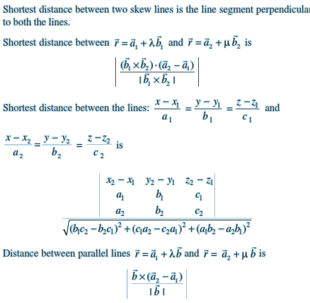
Skew lines are lines in space which are neither parallel nor intersecting. They lie in different planes.

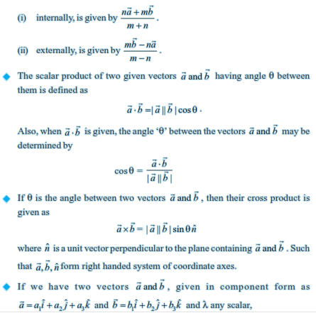
Angle between skew lines is the angle between two intersecting lines drawn from any point (preferably through the origin) parallel to each of the skew lines.

If l₁,m₁,n₁ and l₂,m₂,n₂ are the direction cosines of two lines; and θ is the acute angle between the two lines; then
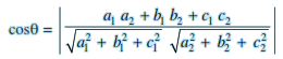
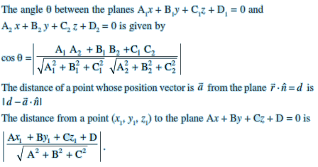
cos θ = | $l_1l_2 + m_1m_2 + n_1n_2$|

If a₁,b₁,c₁ and a₂,b₂,c₂ are the direction ratios of two lines and θ is the acute angle between the two lines; then

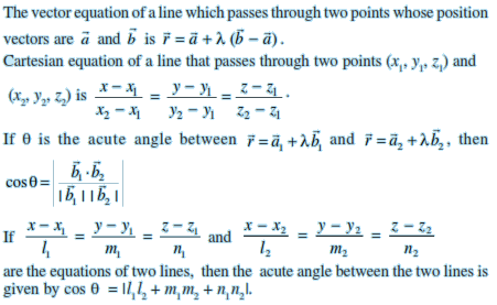
Vector equation of a line that passes through the given point whose position vector is $\overrightarrow{a}$ and parallel to a given vector $\overrightarrow{b}$ is $\overrightarrow{r} = \overrightarrow{a} + \lambda * \overrightarrow{b}$

Equation of a line through a point (x₁,y₁,z₁) and having direction cosines l, m, n is $\frac{x - x_1}{l} = \frac{y - y_1}{m} = \frac{z - z_1}{n}$

In the vector form, equation of a plane which is at a distance d from the origin, and $\hat{n}$ is the unit vector normal to the plane through the origin is $\vec{r}.\hat{n} = d$

Equation of a plane which is at a distance of d from the origin and the direction cosines of the normal to the plane as l, m, n is lx + my + nz = d.

The equation of a plane through a point whose position vector is $\vec{a}$ and perpendicular to the vector $\vec{N}$ is ( $\vec{r}$ - $\vec{a}$ ) . $\vec{N}$ = 0

Equation of a plane perpendicular to a given line with direction ratios A, B, C and passing through a given point (x₁,y₁,z₁) is $A(x - x_1) + B(y - y_1) + C(z - z_1) = 0$

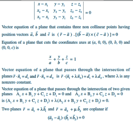
Equation of a plane passing through three non collinear points (x₁,y₁,z₁) , (x₂,y₂,z₂) and (x₃,y₃,z₃) is

Position vector of a point P(x, y, z) is given as $\overrightarrow{OP}$ = $\overrightarrow{r}$ = $x\hat{i} + y\hat{j} + z\hat{k}$ , and its magnitude by $\sqrt{x^2 + y^2 + z^2}$

The scalar components of a vector are its direction ratios, and represent its projections along the respective axes.

The magnitude (r), direction ratios (a, b, c) and direction cosines (l, m, n) of any vector are related as: $l = \frac{a}{r}$ , $m = \frac{b}{r}$ , $n = \frac{c}{r}$

The vector sum of the three sides of a triangle taken in order is $\overrightarrow{0}$

The vector sum of two coinitial vectors is given by the diagonal of the parallelogram whose adjacent sides are the given vectors.

The multiplication of a given vector by a scalar Λ, changes the magnitude of the vector by the multiple | Λ|, and keeps the direction same (or makes it opposite) according as the value of Λ is positive (or negative).

For a given vector $\overrightarrow{a}$, the vector $\hat{a} = \frac{\overrightarrow{a}}{| \overrightarrow{a} | }$ gives the unit vector in the direction of $\hat{a}$

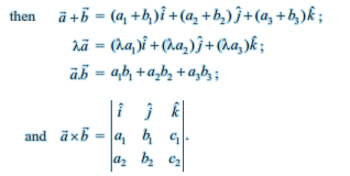
The position vector of a point R dividing a line segment joining the points P and Q whose position vectors are $\overrightarrow{a}$ and $\overrightarrow{b}$ respectively,. in the ratio m : n

A linear programming problem is one that is concerned with finding the optimal value (maximum or minimum) of a linear function of several variables (called objective function) subject to the conditions that the variables are non-negative and satisfy a set of linear inequalities (called linear constraints). Variables are sometimes called decision variables and are non-negative.

A few important linear programming problems are: (i) Diet problems (ii) Manufacturing problems (iii) Transportation problems

The common region determined by all the constraints including the non-negative constraints x ≥ 0, y ≥ 0 of a linear programming problem is called the feasible region (or solution region) for the problem.

Points within and on the boundary of the feasible region represent feasible solutions of the constraints. Any point outside the feasible region is an infeasible solution.

Any point in the feasible region that gives the optimal value (maximum or minimum) of the objective function is called an optimal solution.

Theorem 1 Let R be the feasible region (convex polygon) for a linear programming problem and let Z = ax + by be the objective function. When Z has an optimal value (maximum or minimum), where the variables x and y are subject to constraints described by linear inequalities, this optimal value must occur at a corner point (vertex) of the feasible region.

Theorem 2 Let R be the feasible region for a linear programming problem, and let Z = ax + by be the objective function. If R is bounded, then the objective function Z has both a maximum and a minimum value on R and each of these occurs at a corner point (vertex) of R.

If the feasible region is unbounded, then a maximum or a minimum may not exist. However, if it exists, it must occur at a corner point of R.

Corner point method for solving a linear programming problem. The method comprises of the following steps:

If the feasible region is unbounded, then

If two corner points of the feasible region are both optimal solutions of the same type, i.e., both produce the same maximum or minimum, then any point on the line segment joining these two points is also an optimal solution of the same type.

The salient features of the chapter are –

If E and F are independent, then

Theorem of total probability

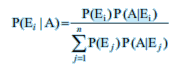
Bayes Theorem

A random variable is a real valued function whose domain is the sample space of a random experiment.

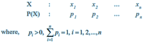
The probability distribution of a random variable X is the system of numbers

Let X be a random variable whose possible values $x_1, x_2, x_3, ... , x_n$ occur with probabilities $p_1, p_2, p_3, ... , p_n$ respectively. The mean of X, denoted by $\mu$, is the number $\sum_{i=1}^n x_i \cdot p_i$. The mean of a random variable X is also called the expectation of X, denoted by E (X).

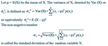
Let X be a random variable whose possible values $x_1, x_2, x_3, ... , x_n$ occur with probabilities $p(x_1), p(x_2), p(x_3), ... , p(x_n)$ respectively.

Var (X) = E (X²) – [E(X)]²

Trials of a random experiment are called Bernoulli trials, if they satisfy the following conditions :