In the previous section, you saw how you can use mini-batch gradient descent to start making progress and start taking gradient descent steps, even when you're just partway through processing your training set even for the first time.

In this section, you learn more details of how to implement gradient descent and gain a better understanding of what it's doing and why it works.

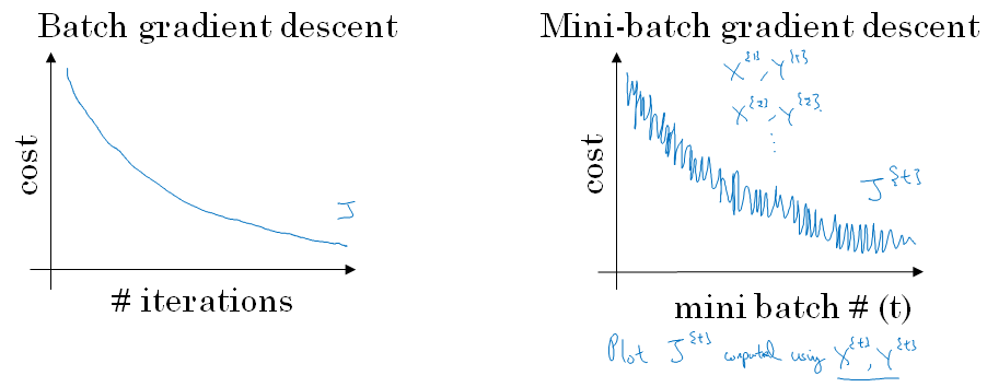
With batch gradient descent on every iteration you go through the entire training set and you'd expect the cost to go down on every single iteration.

So if we've had the cost function j as a function of different iterations it should decrease on every single iteration.

And if it ever goes up even on any iteration then something is wrong. Maybe you're learning rate is too big.

On mini batch gradient descent though, if you plot progress on your cost function, then it may not decrease on every iteration.

In particular, on every iteration you're processing some \(X^{t}, Y^{t}\) and so if you plot the cost function \(J^{t}\), which is computed using just \(X^{t}, Y^{t}\).

Then it's as if on every iteration you're training on a different training set or really training on a different mini batch. So you plot the cost function J, you're more likely to see something that looks like shown below. It should trend downwards, but it's also going to be a little bit noisier.

So if you plot \(J^{t}\), as you're training mini batch in descent it may be over multiple epochs, you might expect to see a curve like shown above.

So it's okay if it doesn't go down on every derivation. But it should trend downwards, and the reason it'll be a little bit noisy is that, maybe \(X^{1}, Y^{1}\) is just the rows of easy mini batch so your cost might be a bit lower, but then maybe just by chance, \(X^{2}, Y^{2}\) is just a harder mini batch.

Maybe you needed some mislabeled examples in it, in which case the cost will be a bit higher and so on. So that's why you get these oscillations as you plot the cost when you're running mini batch gradient descent.

Now one of the parameters you need to choose is the size of your mini batch. So m was the training set size on one extreme, if the mini-batch size, = m, then you just end up with batch gradient descent.

Alright, so in this extreme you would just have one mini-batch \(X^{1}, Y^{1}\) , and this mini-batch is equal to your entire training set. So setting a mini-batch size m just gives you batch gradient descent. The other extreme would be if your mini-batch size, Were = 1.

This gives you an algorithm called stochastic gradient descent.

And here every example is its own mini-batch.

So what you do in this case is you look at the first mini-batch, so X{1}, Y{1}, but when your mini-batch size is one, this just has your first training example, and you take derivative to sense that your first training example.

And then you next take a look at your second mini-batch, which is just your second training example, and take your gradient descent step with that, and then you do it with the third training example and so on looking at just one single training sample at the time.

So let's look at what these two extremes will do on optimizing this cost function.

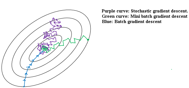
If these are the contours of the cost function you're trying to minimize so your minimum is at the center as shown in below figure. Then batch gradient descent might start somewhere and be able to take relatively low noise, relatively large steps. And you could just keep matching to the minimum.

In contrast with stochastic gradient descent If you start somewhere at a different starting point. Then on every iteration you're taking gradient descent with just a single training example so most of the time you hit at the global minimum.

But sometimes you hit in the wrong direction if that one example happens to point you in a bad direction. So stochastic gradient descent can be extremely noisy.

And on average, it'll take you in a good direction, but sometimes it'll head in the wrong direction as well.

As stochastic gradient descent won't ever converge, it'll always just kind of oscillate and wander around the region of the minimum. But it won't ever just head to the minimum and stay there.

In practice, the mini-batch size you use will be somewhere in between.

Somewhere between in 1 and m and 1 and m are respectively too small and too large. And here's why. If you use batch grading descent, So this is your mini batch size equals m.

Then you're processing a huge training set on every iteration. So the main disadvantage of this is that it takes too much time too long per iteration assuming you have a very long training set.

If you have a small training set then batch gradient descent is fine. If you go to the opposite, if you use stochastic gradient descent,

Then it's nice that you get to make progress after processing just one example that's actually not a problem. And the noisiness can be ameliorated or can be reduced by just using a smaller learning rate. But a huge disadvantage to stochastic gradient descent is that you lose almost all your speed up from vectorization.

Because, here you're processing a single training example at a time. The way you process each example is going to be very inefficient. So what works best in practice is something in between where you have some,

Mini-batch size not to big or too small.

And this gives you in practice the fastest learning.

And you notice that this has two good things going for it. One is that you do get a lot of vectorization.

So in the example we used on the previous section, if your mini batch size was 1000 examples then, you might be able to vectorize across 1000 examples which is going to be much faster than processing the examples one at a time.

And second, you can also make progress, Without needing to wait till you process the entire training set.

So again using the numbers we have from the previous section, each epoch of your training set allows you to see 5,000 gradient descent steps.

So in practice they'll be some in-between mini-batch size that works best. And so with mini-batch gradient descent we'll start and maybe It's not guaranteed to always head toward the minimum but it tends to head more consistently in direction of the minimum than the stochastic gradient descent.

And then it doesn't always exactly converge or oscillate in a very small region.

If that's an issue you can always reduce the learning rate slowly. We'll talk more about learning rate decay or how to reduce the learning rate in a later section.

So if the mini-batch size should not be m and should not be 1 but should be something in between, how do you go about choosing it? Well, here are some guidelines. First, if you have a small training set, Just use batch gradient descent.

If you have a small training set then no point using mini-batch gradient descent you can process a whole training set quite fast. So you might as well use batch gradient descent.

What a small training set means, I would say if it's less than maybe 2000 it'd be perfectly fine to just use batch gradient descent. Otherwise, if you have a bigger training set, typical mini batch sizes would be, Anything from 64 up to maybe 512 are quite typical.

And because of the way computer memory is layed out and accessed, sometimes your code runs faster if your mini-batch size is a power of 2.

One last tip is to make sure that your mini batch, fits in CPU/GPU memory.

And this really depends on your application and how large a single training sample is. But if you ever process a mini-batch that doesn't actually fit in CPU, GPU memory, Then you find that the performance suddenly falls of a cliff and is suddenly much worse.

So I hope this gives you a sense of the typical range of mini batch sizes that people use.

In practice of course the mini batch size is another hyper parameter that you might do a quick search over to try to figure out which one is most sufficient of reducing the cost function j.

So what i would do is just try several different values. Try a few different powers of two and then see if you can pick one that makes your gradient descent optimization algorithm as efficient as possible.

But hopefully this gives you a set of guidelines for how to get started with that hyper parameter search. You now know how to implement mini-batch gradient descent and make your algorithm run much faster, especially when you're training on a large training set.

But it turns out there're even more efficient algorithms than gradient descent or mini-batch gradient descent. Let's start talking about them in the next few sections.