In the last section, we saw exponentially weighted averages. This will turn out to be a key component of several optimization algorithms that you used to train your neural networks.

So, in this section, we delve a little bit deeper into intuitions for what this algorithm is really doing.

Recall that this is a key equation for implementing exponentially weighted averages \( V_t = \beta V_{t-1} + (1 - \beta) \theta_t \).

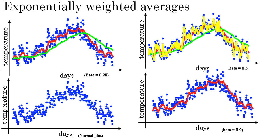
And so, if beta equals 0.9 you got the red line. If it was much closer to one, if it was 0.98, you get the green line. And it it's much smaller, maybe 0.5, you get the yellow line.

Let's look a bit more than that to understand how this is computing averages of the daily temperature.

So here's that equation again, and let's set beta equals 0.9 and write out a few equations that this corresponds to.

So whereas, when you're implementing it you have T going from zero to one, to two to three, increasing values of T. To analyze it, I've written it with decreasing values of T.

\( V_{100} = 0.9V_{99} + 0.1\theta_{100} \\ V_{99} = 0.9V_{98} + 0.1\theta_{99} \\ V_{98} = 0.9V_{97} + 0.1\theta_{98} \\ . \\ . \\ . \\ . \\ V_t = 0.9V_{t-1} + 0.1\theta_t \)

\( V_{100} = 0.9V_{99} + 0.1\theta_{100} \\ V_{100} = 0.1\theta_{100} + 0.9 (0.9V_{98} + 0.1\theta_{99} )\\ V_{100} = 0.1\theta_{100} + (0.9 * 0. 1)(\theta_{99}) + (0.9 * 0.9)(V_{98}) \\ V_{100} = 0.1\theta_{100} + (0.9 * 0. 1)(\theta_{99}) + (0.9)^2 (0.9V_{97} + 0.1\theta_{98}) \\ . \\ . \\ . \\ . \\ V_{100} = 0.1\theta_{100} + (0.9 * 0. 1)(\theta_{99}) + (0.1)(0.9)^2(\theta_{98}) + (0.1)(0.9)^3(\theta_{97}) + (0.1)(0.9)^4(\theta_{96}) + ... \)

So this is really a way to sum and that's a weighted average of \( \theta_{100} \), which is the current days temperature and we're looking for a perspective of \( V_{100} \) which you calculate on the 100th day of the year.

But those are sum of your \( \theta_{100}, \theta_{99}, \theta_{98}, \theta_{97}, \theta_{96} ... \), and so on.

So one way to draw this in pictures would be if, let's say we have some number of days of temperature.

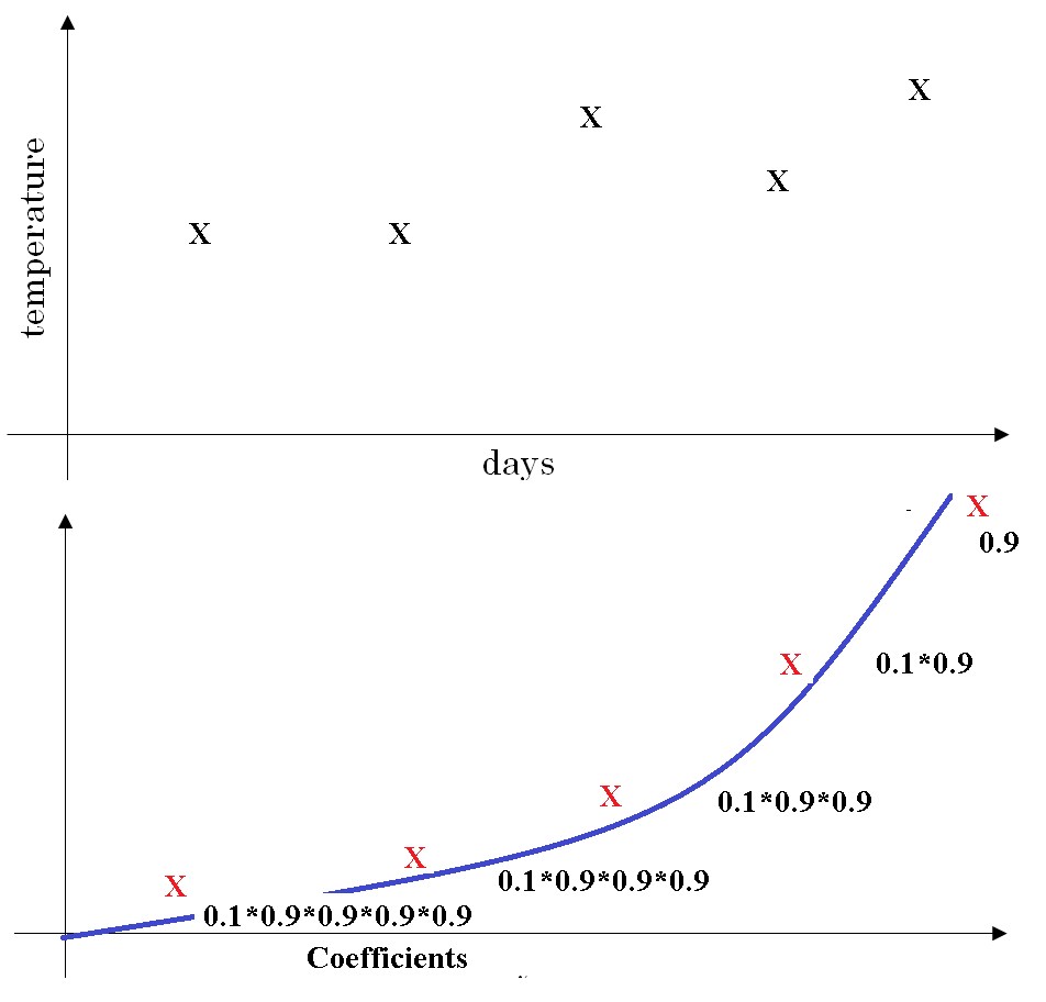
So t = 5 in above figure, and \( \theta \) and the corresponding coefficients are given. The chart on top gives \( \theta_4, \theta_3, \theta_2, \theta_1, \theta_0 \)

And what we have is then an exponentially decaying function \( 0.1 , 0.1*0.9, 0.1*(0.9)^2, 0.1*(0.9)^3, 0.1*(0.9)^4\) So you have this exponentially decaying function.

And the way you compute V₅, is you take the element wise product between these two functions and sum it up.

So it's really taking the daily temperature, multiply with this exponentially decaying function, and then summing it up. And this becomes your V₅.

It turns out that all of these coefficients, add up to one or add up to very close to one. But because of that, this really is an exponentially weighted average.

So when beta equals 0.9 \( \frac{1}{1 - \beta} = 10\), we say that, this is as if you're computing an exponentially weighted average that focuses on just the last 10 days temperature.

Finally, let's talk about how you actually implement this.

Vθ = 0

Repeat {

Get next θt

Vθ = β Vθ + (1 - β) θt

}

So one of the advantages of this exponentially weighted average formula, is that it takes very little memory.

You just need to keep just one row number in computer memory, and you keep on overwriting it with this formula based on the latest values that you got. And it's really this reason, the efficiency, it just takes up one line of code basically and just storage and memory for a single row number to compute this exponentially weighted average.

It's really not the best way, not the most accurate way to compute an average. If you were to compute a moving window, where you explicitly sum over the last 10 days, the last 50 days temperature and just divide by 10 or divide by 50, that usually gives you a better estimate.

But the disadvantage of that, of explicitly keeping all the temperatures around and sum of the last 10 days is it requires more memory, and it's just more complicated to implement and is computationally more expensive.

So for things, we'll see some examples on the next few videos, where you need to compute averages of a lot of variables. This is a very efficient way to do so both from computation and memory efficiency point of view which is why it's used in a lot of machine learning.

Not to mention that there's just one line of code which is, maybe, another advantage.

So, now, you know how to implement exponentially weighted averages.

There's one more technical detail that's worth for you knowing about called bias correction. Let's see that in the next video, and then after that, you will use this to build a better optimization algorithm than the straight forward create