In terms of designing content architectures, one of the ideas that really helps is using a one by one convolution.

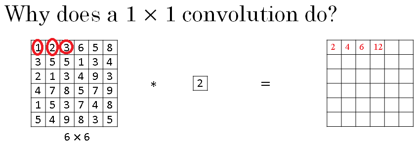
Now, you might be wondering, what does a one by one convolution do? Isn't that just multiplying by numbers? That seems like a funny thing to do. Turns out it's not quite like that. Let's take a look.

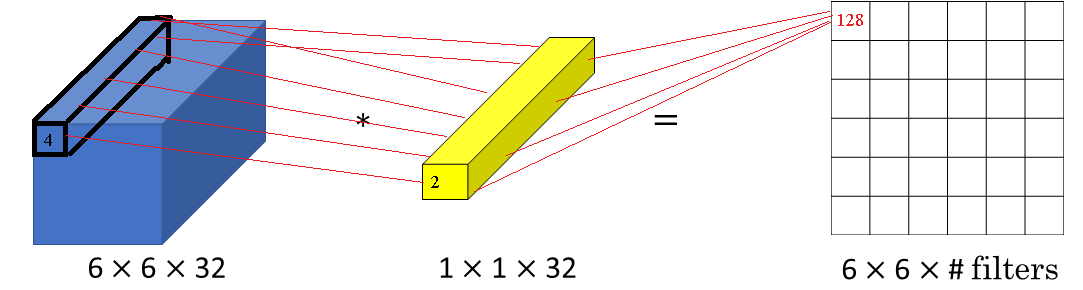
In this we have a one by one filter, we'll put in number two there, and if you take the six by six by one and convolve it with this one by one by one filter, you end up just taking the image and multiplying it by two.

So, one, two, three ends up being two, four, six, and so on. And so, a convolution by a one by one filter, doesn't seem particularly useful.

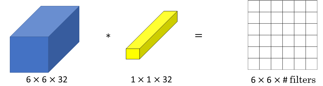
You just multiply it by some number. But that's the case of six by six by one channel images. If you have a 6 by 6 by 32 instead of by 1, then a convolution with a 1 by 1 filter can do something that makes much more sense.

And in particular, what a one by one convolution will do in the above case is it will look at each of the 36 different positions of the image given above, and it will take the element wise product between 32 numbers and 32 numbers in the filter. And then apply a ReLU non-linearity to it after that.

So, to look at one of the 36 positions, maybe one slice through this value, you take these 36 numbers multiply it by 1 slice through the volume like that, and you end up with a single real number which then gets plotted in one of the outputs like shown below.

And in fact, one way to think about the 32 numbers you have in this 1 by 1 by 32 filters is that, it's as if you have neuron that is taking as input, 32 numbers multiplying each of these 32 numbers in one slice of the image with by 32 different channels, multiplying them by 32 weights and then applying a ReLU non-linearity to it and then outputting the corresponding thing over in the output.

And more generally, if you have not just one filter, but if you have multiple filters, then it's as if you have not just one unit, but multiple units, taken as input all the numbers in one slice, and then building them up into an output of six by six by number of filters.

And this idea is often called a one by one convolution but it's sometimes also called Network in Network, and is described in this paper, by Min Lin, Qiang Chen, and Schuicheng Yan. And even though the details of the architecture in this paper aren't used widely, this idea of a one by one convolution or this sometimes called Network in Network idea has been very influential, has influenced many other neural network architectures including the inception network.

But to give you an example of where one by one convolution is useful, here's something you could do with it.

Let's say you have a 28 by 28 by 192 volume. If you want to shrink the height and width, you can use a pooling layer. So we know how to do that. But one of a number of channels has gotten too big and we want to shrink that. How do you shrink it to a 28 by 28 by 32 dimensional volume?

Well, what you can do is use 32 filters that are one by one. And technically, each filter would be of dimension 1 by 1 by 192, because the number of channels in your filter has to match the number of channels in your input volume, but you use 32 filters and the output of this process will be a 28 by 28 by 32 volume.

So this is a way to let you shrink nc as well, whereas pooling layers, I used just to shrink nH and nW, the height and width these volumes. And we'll see later how this idea of one by one convolutions allows you to shrink the number of channels and therefore, save on computation in some networks.

But of course, if you want to keep the number of channels at 192, that's fine too. And the effect of the one by one convolution is it just adds non-linearity. It allows you to learn the more complex function of your network by adding another layer that inputs 28 by 28 by 192 and outputs 28 by 28 by 192.

So, that's how a one by one convolutional layer is actually doing something pretty non-trivial and adds non-linearity to your neural network and allow you to decrease or keep the same or if you want, increase the number of channels in your volumes. Next, you'll see that this is actually very useful for building the inception network.

Let's go on to that in the next video. So, you've now seen how a one by one convolution operation is actually doing a pretty non-trivial operation and it allows you to shrink the number of channels in your volumes or keep it the same or even increase it if you want.

When designing a layer for a ConvNet, you might have to pick, do you want a 1 by 1 filter, or 3 by 3, or 5 by 5, or do you want a pooling layer?

What the inception network does is it says, why should you do them all? And this makes the network architecture more complicated, but it also works remarkably well. Let's see how this works.

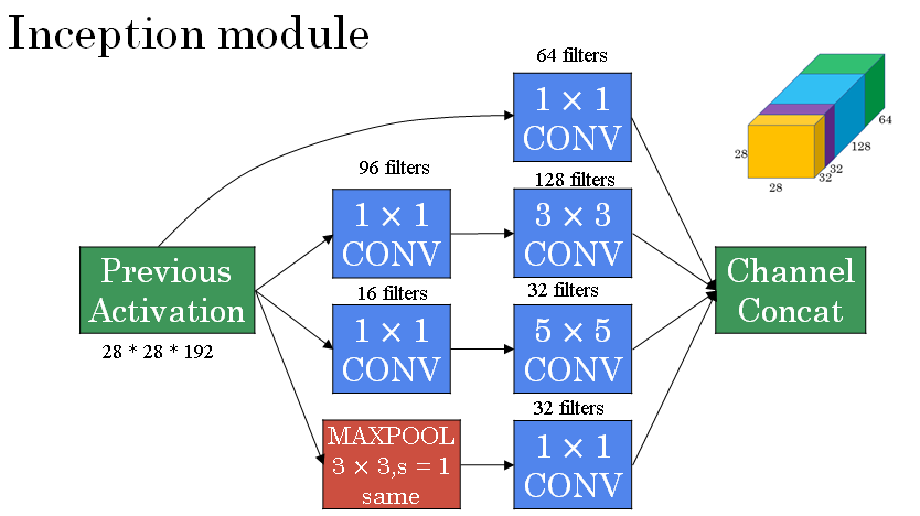
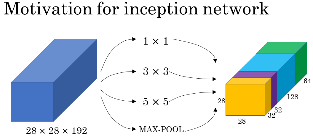
Let's say for the sake of example that you have inputted a 28 by 28 by 192 dimensional volume. So what the inception network or what an inception layer says is, instead choosing what filter size you want in a Conv layer, or even do you want a convolutional layer or a pooling layer? Let's do them all.

So what if you can use a 1 by 1 convolution, and that will output a 28 by 28 by something. Let's say 28 by 28 by 64 output, and you just have a volume there.

But maybe you also want to try a 3 by 3 and that might output a 20 by 20 by 128.

And then what you do is just stack up this second volume next to the first volume.

And to make the dimensions match up, let's make this a same convolution. So the output dimension is still 28 by 28, same as the input dimension in terms of height and width.

But 28 by 28 by in this example 128. And maybe you might say well I want to hedge my bets. Maybe a 5 by 5 filter works better. So let's do that too and have that output a 28 by 28 by 32.

And again you use the same convolution to keep the dimensions the same.

And maybe you don't want to convolutional layer. Let's apply pooling, and that has some other output and let's stack that up as well. And here pooling outputs 28 by 28 by 32.

Now in order to make all the dimensions match, you actually need to use padding for max pooling. So this is an unusual form of pooling because if you want the input to have a higher than 28 by 28 and have the output, you'll match the dimension everything else also by 28 by 28, then you need to use the same padding as well as a stride of one for pooling.

So this detail might seem a bit funny to you now, but let's keep going. And we'll make this all work later. But with a inception module like this, you can input some volume and output.

In this case I guess if you add up all these numbers, 32 plus 32 plus 128 plus 64, that's equal to 256. So you will have one inception module input 28 by 28 by 129, and output 28 by 28 by 256.

And this is the heart of the inception network which is due to Christian Szegedy, Wei Liu, Yangqing Jia, Pierre Sermanet, Scott Reed, Dragomir Anguelov, Dumitru Erhan, Vincent Vanhoucke and Andrew Rabinovich.

And the basic idea is that instead of you needing to pick one of these filter sizes or pooling you want and committing to that, you can do them all and just concatenate all the outputs, and let the network learn whatever parameters it wants to use, whatever the combinations of these filter sizes it wants.

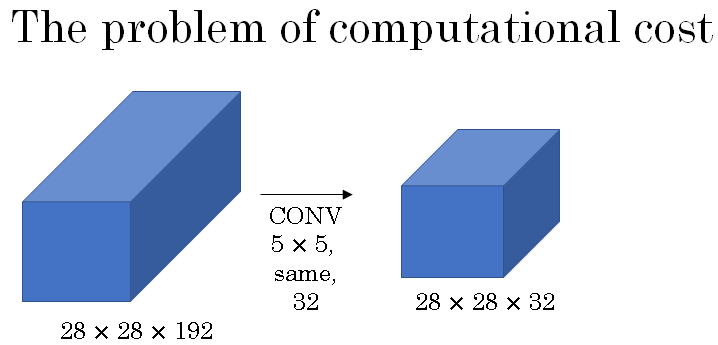
Now it turns outthat there is a problem with the inception layer as we've described it here, which is computational cost.

Let's figure out what's the computational cost of a 5 by 5 filter resulting in a block in the inception network.

So just focusing on the 5 by 5 block we had as input a 28 by 28 by 192 block, and you implement a 5 by 5 same convolution of 32 filters to output 28 by 28 by 32.

Let's look at the computational costs of outputting this 20 by 20 by 32. You have 32 filters because the outputs has 32 channels, and each filter is going to be 5 by 5 by 192. And so the output size is 20 by 20 by 32, and so you need to compute 28 by 28 by 32 numbers.

The total number of multiplies you need is the number of multiplies you need to compute each of the output values times the number of output values you need to compute. And if you multiply all of these numbers, this is equal to 120 million.

And so, while you can do 120 million multiplies on the modern computer, this is still a pretty expensive operation.

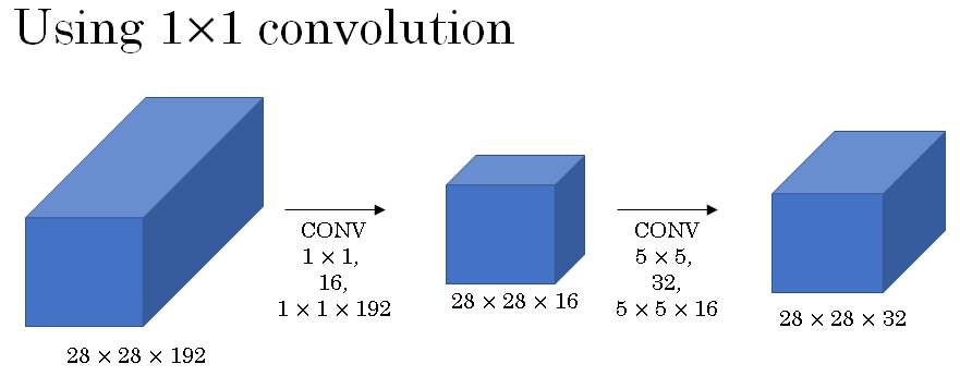
By using the idea of 1 by 1 convolutions, which you learnt you'll be able to reduce the computational costs by about a factor of 10. To go from about 120 million multiplies to about one tenth of that.

Here is an alternative architecture for inputting 28 by 28 by 192, and outputting 28 by 28 by 32. You are going to input the volume, use a 1 by 1 convolution to reduce the volume to 16 channels instead of 192 channels, and then on this much smaller volume, run your 5 by 5 convolution to give you your final output.

So notice the input and output dimensions are still the same. You input 28 by 28 by 192 and output 28 by 28 by 32, same as the previous section.

But what we've done is we're taking this huge volume we had on the left, and we shrunk it to this much smaller intermediate volume, which only has 16 instead of 192 channels. Sometimes this is called a bottleneck laye

We shrink the representation before increasing the size again.

Now let's look at the computational costs involved. To apply this 1 by 1 convolution, we have 16 filters. Each of the filters is going to be of dimension 1 by 1 by 192, this 192 matches that 192. And so the cost of computing this 28 by 28 by 16 volumes is going to be about 2.4 million.

The cost of this second convolutional layer would be that well, you have these many outputs. So 28 by 28 by 32. And then for each of the outputs you have to apply a 5 by 5 by 16 dimensional filter. And so by 5 by 5 by 16. And you multiply that out is equals to 10.0 million. And so the total number of multiplications you need to do is the sum of those which is 12.4 million multiplications.

And you compare this with what we had on the previous section, you reduce the computational cost from about 120 million multiplies, down to about one tenth of that, to 12.4 million multiplications. And the number of additions you need to do is about very similar to the number of multiplications you need to do.

So that's why I'm just counting the number of multiplications. So to summarize, if you are building a layer of a neural network and you don't want to have to decide, do you want a 1 by 1, or 3 by 3, or 5 by 5, or pooling layer, the inception module let's you say let's do them all, and let's concatenate the results.

And then we run to the problem of computational cost.

And what you saw here was how using a 1 by 1 convolution, you can create this bottleneck layer thereby reducing the computational cost significantly.

Now you might be wondering, does shrinking down the representation size so dramatically, does it hurt the performance of your neural network?

It turns out that so long as you implement this bottleneck layer so that within reason, you can shrink down the representation size significantly, and it doesn't seem to hurt the performance, but saves you a lot of computation.

So these are the key ideas of the inception module. Let's put them together and in the next section show you what the full inception network looks like.

In a previous section, you've already seen all the basic building blocks of the Inception network. In this section, let's see how you can put these building blocks together to build your own Inception network.

The inception module takes as input the activation or the output from some previous layer.

So let's say for the sake of argument this is 28 by 28 by 192, same as our previous section. The example we worked through in depth was the 1 by 1 followed by 5 by 5.

Then to save computation on your 3 by 3 convolution you can also do the same here. And then the 3 by 3 outputs, 28 by 28 by 128.

And then maybe you want to consider a 1 by 1 convolution as well. There's no need to do a 1 by 1 conv followed by another 1 by 1 conv so there's just one step here and let's say these outputs 28 by 28 by 64. And then finally is the pooling layer.

So here I'm going to do something funny. In order to really concatenate all of these outputs at the end we are going to use the same type of padding for pooling. So that the output height and width is still 28 by 28. So we can concatenate it with these other outputs.

But notice that if you do max-pooling, even with same padding, 3 by 3 filter is tried at 1. The output here will be 28 by 28, By 192.

It will have the same number of channels and the same depth as the input that we had here. So, this seems like is has a lot of channels.

So what we're going to do is actually add one more 1 by 1 conv layer and it gets us down to 28 by 28 by 32. And the way you do that, is to use 32 filters, of dimension 1 by 1 by 192. So that's why the output dimension has a number of channels shrunk down to 32. So then we don't end up with the pooling layer taking up all the channels in the final output.

And finally you take all of these blocks and you do channel concatenation. Just concatenate across this 64 plus 128 plus 32 plus 32 and this if you add it up this gives you a 28 by 28 by 256 dimension output. Concat is just this concatenating the blocks that we saw in the previous section.

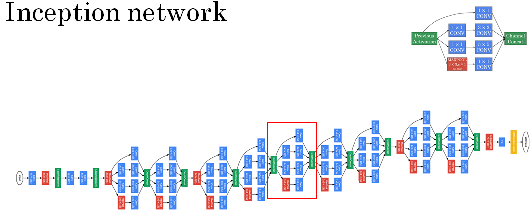
So this is one inception module, and what the inception network does, is, more or less, put a lot of these modules together.

Here's a picture of the inception network, taken from the paper by Szegedy et al And you notice a lot of repeated blocks in this. Maybe this picture looks really complicated. But if you look at one of the blocks there, that block is basically the inception module that you saw on the previous section.

The inception network is just a lot of these blocks that you've learned about repeated to different positions of the network. But so you understand the inception block from the previous section, then you understand the inception network.