In the last section, you learned how to use a convolutional implementation of sliding windows. That's more computationally efficient, but it still has a problem of not quite outputting the most accurate bounding boxes.

In this section, let's see how you can get your bounding box predictions to be more accurate.

With sliding windows, you take sets of locations and run the classifier through it. And in this case, none of the boxes really match up perfectly with the position of the car.

So, maybe that box is the best match. And also, it looks like in drawn through, the perfect bounding box isn't even quite square, it's actually has a slightly wider rectangle or slightly horizontal aspect ratio.

So, is there a way to get this algorithm to outputs more accurate bounding boxes? A good way to get this output more accurate bounding boxes is with the YOLO algorithm.

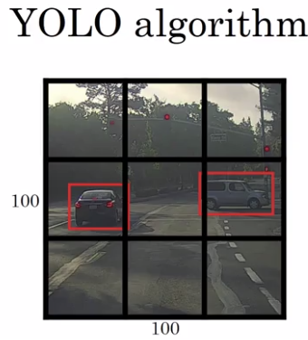
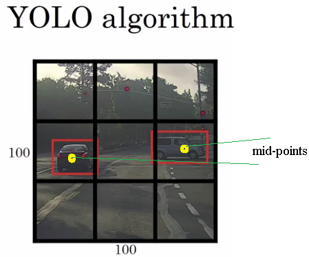
YOLO stands for, You Only Look Once. And is an algorithm due to Joseph Redmon, Santosh Divvala, Ross Girshick and Ali Farhadi. Here's what you do. Let's say you have an input image at 100 by 100, you're going to place down a grid on this image. And for the purposes of illustration, I'm going to use a 3 by 3 grid. Although in an actual implementation, you use a finer one, like maybe a 19 by 19 grid.

And the basic idea is you're going to take the image classification and localization algorithm that you saw a few sections back, and apply it to each of the nine grids.

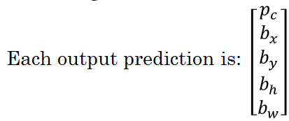
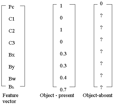
So for each of the nine grid cells, you specify a label Y, where the label Y is this eight dimensional vector, same as you saw previously. Your first output P_c = {0, 1} depending on whether or not there's an image in that grid cell and then B_x, B_y, B_h, B_w to specify the bounding box if there is an image, if there is an object associated with that grid cell. And then say, C₁, C₂, C₃, if you try and recognize three classes not counting the background class.

So you try to recognize pedestrian's class, motorcycles and the background class. Then C₁, C₂, C₃ can be the pedestrian, car and motorcycle classes.

So in this image, we have nine grid cells, so you have a vector like this for each of the grid cells. So let's start with the upper left grid cell. For that one, there is no object. So, the label vector Y for the upper left grid cell would be zero, and then don't cares for the rest of these.

Now, how about a grid cell with an object? To give a bit more detail, this image has two objects. And what the YOLO algorithm does is it takes the midpoint of each of the two objects and then assigns the object to the grid cell containing the midpoint. So the left car is assigned to one grid cell, and the car on the right is assigned to another grid cell.

And so even though the central grid cell has some parts of both cars, we'll pretend the central grid cell has no interesting object so that the central grid cell the class label Y also looks like a vector with no object - the first component PC, and then the rest are don't cares.

So, for each of these nine grid cells, you end up with a eight dimensional output vector. And because you have 3 by 3 grid cells, you have nine grid cells, the total volume of the output is going to be 3 by 3 by 8.

So the target output is going to be 3 by 3 by 8 because you have 3 by 3 grid cells. And for each of the 3 by 3 grid cells, you have a eight dimensional Y vector. So the target output volume is 3 by 3 by 8.

Now, to train your neural network, the input is 100 by 100 by 3, that's the input image. And then you have a usual convnet with conv layers of max pool layers, and so on. So that in the end this eventually maps to a 3 by 3 by 8 output volume.

And so what you do is you have an input X which is the input image like that, and you have these target labels Y which are 3 by 3 by 8, and you use back propagation to train the neural network to map from any input X to this type of output volume Y.

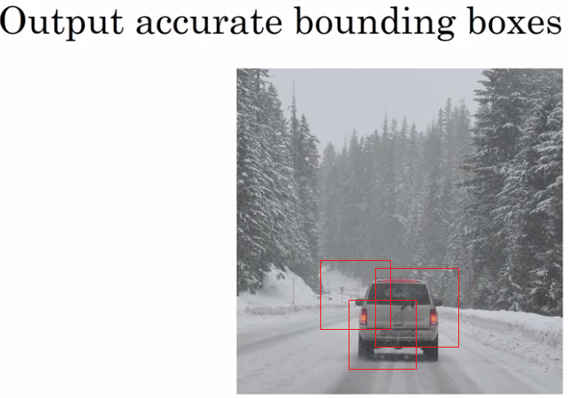
So the advantage of this algorithm is that the neural network outputs precise bounding boxes as follows. So at test time, what you do is you feed an input image X and run forward prop until you get this output Y. And then for each of the nine outputs of each of the 3 by 3 positions in which of the output, you can then just read off 1 or 0.

Is there an object associated with that one of the nine positions? And that there is an object, what object it is, and where is the bounding box for the object in that grid cell? And so long as you don't have more than one object in each grid cell, this algorithm should work okay.

And the problem of having multiple objects within the grid cell is something we'll address later.

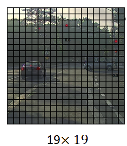
If we use a relatively small 3 by 3 grid, in practice, you might use a much finer, grid maybe 19 by 19. So you end up with 19 by 19 by 8, and that also makes your grid much finer. It reduces the chance that there are multiple objects assigned to the same grid cell.

And just as a reminder, the way you assign an object to grid cell is you look at the midpoint of an object and then you assign that object to whichever one grid cell contains the midpoint of the object.

So each object, even if the objects spends multiple grid cells, that object is assigned only to one of the nine grid cells, or one of the 3 by 3, or one of the 19 by 19 grid cells.

The chance of an object of two midpoints of objects appearing in the same grid cell is just a bit smaller. So notice two things, first, this is a lot like the image classification and localization algorithm that we talked about in the first section.

And that it outputs the bounding boxes coordinates explicitly. And so this allows in your network to output bounding boxes of any aspect ratio, as well as, output much more precise coordinates that aren't just dictated by the stripe size of your sliding windows classifier.

And second, this is a convolutional implementation and you're not implementing this algorithm nine times on the 3 by 3 grid or if you're using a 19 by 19 grid.19 squared is 361. So, you're not running the same algorithm 361 times or 19 squared times. Instead, this is one single convolutional implantation, where you use one ConvNet with a lot of shared computation between all the computations needed for all of your 3 by 3 or all of your 19 by 19 grid cells.

So, this is a pretty efficient algorithm. And in fact, one nice thing about the YOLO algorithm, which is constant popularity is because this is a convolutional implementation, it actually runs very fast. So this works even for real time object detection.

Now, before wrapping up, there's one more detail I want to share with you, which is, how do you encode these bounding boxes bx, by, BH, BW? Let's discuss that.

So, given these two cars, remember, we have the 3 by 3 grid.

Let's take the example of the car below.

So, in this grid cell there is an object and so the target label y will be one, that was PC is equal to one. So, how do you specify the bounding box?

In the YOLO algorithm, relative to this square, when I take the convention that the upper left point here is 0 0 and this lower right point is 1 1. So to specify the position of that midpoint, that orange dot, bx might be, let's say x looks like is about 0.4. Maybe its about 0.4 of the way to their right. And then y, looks I guess maybe 0.3. And then the height of the bounding box is specified as a fraction of the overall width of this box.

So, the width of this red box is maybe 90% of that blue line.

And so BH is 0.9 and the height of this is maybe one half of the overall height of the grid cell. So in that case, BW would be, let's say 0.5.

So, in other words, this bx, by, bh, bw as specified relative to the grid cell. And so bx and by, this has to be between 0 and 1.

So, there are multiple ways of specifying the bounding boxes, but this would be one convention that's quite reasonable.

So, that's it for the YOLO or the You Only Look Once algorithm. And in the next few section I'll show you a few other ideas that will help make this algorithm even better. In the meantime, if you want, you can take a look at YOLO paper reference at the bottom of these past couple slides I use.

Although, just one warning, if you take a look at these papers which is the YOLO paper is one of the harder papers to read. I remember, when I was reading this paper for the first time, I had a really hard time figuring out what was going on.

And I wound up asking a couple of my friends, very good researchers to help me figure it out, and even they had a hard time understanding some of the details of the paper.

So, if you look at the paper, it's okay if you have a hard time figuring it out.

I wish it was more uncommon, but it's not that uncommon, sadly, for even senior researchers, that review research papers and have a hard time figuring out the details.

And have to look at open source code, or contact the authors, or something else to figure out the details of these outcomes.

But don't let me stop you from taking a look at the paper yourself though if you wish, but this is one of the harder ones. So, that though, you now understand the basics of the YOLO algorithm. Let's go on to some additional pieces that will make this algorithm work even better.

So how do you tell if your object detection algorithm is working well? In this section, you'll learn about a function called, "Intersection Over Union".

And as we use it both for evaluating your object detection algorithm, as well as using it to add another component to your object detection algorithm, to make it work even better. Let's get started.

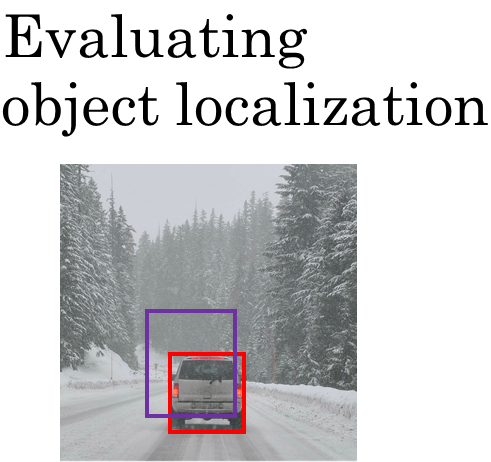
In the object detection task, you expected to localize the object as well. So if that's the ground-truth bounding box, and if your algorithm outputs this bounding box in purple, is this a good outcome or a bad one?

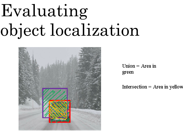
So what the intersection over union function does, or IoU does, is it computes the intersection over union of these two bounding boxes. So, the union of these two bounding boxes is really the area that is contained in either bounding boxes, whereas the intersection is this smaller region contained by both bounding boxes.

So what the intersection of a union does is it computes the size of the intersection. So that yellow shaded area, and divided by the size of the union, which is that green shaded area.

And by convention, the division task will judge that your answer is correct if the IoU is greater than 0.5.

And if the predicted and the ground-truth bounding boxes overlapped perfectly, the IoU would be one, because the intersection would equal to the union. But in general, so long as the IoU is greater than or equal to 0.5, then the answer will look okay.

And by convention, very often 0.5 is used as a threshold to judge as whether the predicted bounding box is correct or not. This is just a convention. If you want to be more stringent, you can judge an answer as correct, only if the IoU is greater than equal to 0.6 or some other number.

But the higher the IoUs, the more accurate the bounding the box. And so, this is one way to map localization, to accuracy where you just count up the number of times an algorithm correctly detects and localizes an object where you could use a definition like this, of whether or not the object is correctly localized.

And again 0.5 is just a human chosen convention. There's no particularly deep theoretical reason for it. You can also choose some other threshold like 0.6 if you want to be more stringent. I sometimes see people use more stringent criteria like 0.6 or maybe 0.7. I rarely see people drop the threshold below 0.5.

Now, what motivates the definition of IoU, as a way to evaluate whether or not your object localization algorithm is accurate or not. But more generally, IoU is a measure of the overlap between two bounding boxes.

Where if you have two boxes, you can compute the intersection, compute the union, and take the ratio of the two areas. And so this is also a way of measuring how similar two boxes are to each other.

And we'll see this use again this way in the next section when we talk about non-max suppression. So that's it for IoU or Intersection over Union.

One of the problems of Object Detection as you've learned about this so far, is that your algorithm may find multiple detections of the same objects.

Rather than detecting an object just once, it might detect it multiple times.

Non-max suppression is a way for you to make sure that your algorithm detects each object only once. Let's go through an example. Let's say you want to detect pedestrians, cars, and motorcycles in this image. You might place a grid over this, and this is a 19 by 19 grid. Now, while technically this car has just one midpoint, so it should be assigned just one grid cell.

And the car on the left also has just one midpoint, so technically only one of those grid cells should predict that there is a car. In practice, you're running an object classification and localization algorithm for every one of these split cells. So it's quite possible that many split cell might think that the center of a car is in it.

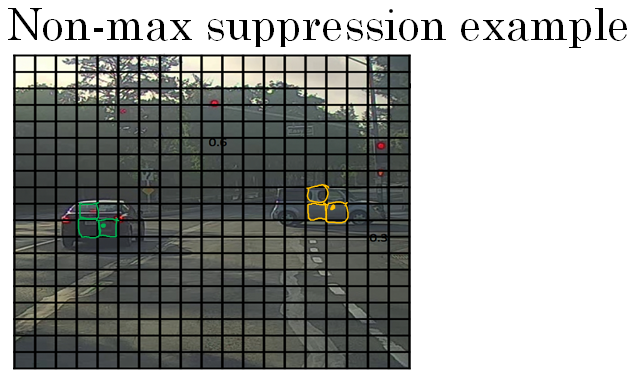
In below example a 19 x 19 grid is placed and so multiple boxes of the grid feel the car is present in them.

Let's step through an example of how non-max suppression will work.

So, what non-max suppression does, is it cleans up these detections. So they end up with just one detection per car, rather than multiple detections per car.

So concretely, what it does, is it first looks at the probabilities associated with each of these detections.

In below image we have multiple detections of the same object. Each detection has a confidence probability associated with it.

let's just say is Pc with the probability of a detection. And it first takes the largest one, which in this case is 0.9 and says, "That's my most confident detection, so let's highlight that and just say I found the car there."

Having done that the non-max suppression part then looks at all of the remaining rectangles and all the ones with a high overlap i.e. with a high IOU will get suppressed.

So those two rectangles with the 0.6 and the 0.7. Both of those overlap a lot with the light blue rectangle. So those, you are going to suppress and darken them to show that they are being suppressed.

Next, you then go through the remaining rectangles for the next car on the left of the image and find the one with the highest probability, the highest Pc, which in this case is this one with 0.8.

So let's commit to that and just say, "Oh, I've detected a car there." And then, the non-max suppression part is to then get rid of any other ones with a high IOU.

So now, every rectangle has been either highlighted or darkened. And if you just get rid of the darkened rectangles, you are left with just the highlighted ones, and these are your two final predictions. So, this is non-max suppression. And non-max means that you're going to output your maximal probabilities classifications but suppress the close-by ones that are non-maximal. Hence the name, non-max suppression.

Let's go through the details of the algorithm. First, on this 19 by 19 grid, you're going to get a 19 by 19 by eight output volume. Although, for this example, I'm going to simplify it to say that you only doing car detection.

So, let me get rid of the C1, C2, C3, and pretend for this example, that each output for each of the 19 by 19, so for each of the 361, which is 19 squared, for each of the 361 positions, you get an output prediction of the following.

Which is the chance there's an object, and then the bounding box. And if you have only one object, there's no C1, C2, C3 prediction.

The details of what happens, you have multiple objects, I'll leave to the programming exercise, which is provided in the course.

Now, to intimate non-max suppression, the first thing you can do is discard all the boxes, discard all the predictions of the bounding boxes with Pc less than or equal to some threshold, let's say 0.6. So we're going to say that unless you think there's at least a 0.6 chance it is an object there, let's just get rid of it. This has caused all of the low probability output boxes.

The way to think about this is for each of the 361 positions, you output a bounding box together with a probability of that bounding box being a good one. So we're just going to discard all the bounding boxes that were assigned a low probability.

Next, while there are any remaining bounding boxes that you've not yet discarded or processed, you're going to repeatedly pick the box with the highest probability, with the highest Pc, and then output that as a prediction.

Next, you then discard any remaining box. Any box that you have not output as a prediction, and that was not previously discarded. So discard any remaining box with a high overlap, with a high IOU, with the box that you just output in the previous step.

And so, you keep doing this while there's still any remaining boxes that you've not yet processed, until you've taken each of the boxes and either output it as a prediction, or discarded it as having too high an overlap, or too high an IOU, with one of the boxes that you have just output as your predicted position for one of the detected objects.

I've described the algorithm using just a single object on this slide. If you actually tried to detect three objects say pedestrians, cars, and motorcycles, then the output vector will have three additional components.

And it turns out, the right thing to do is to independently carry out non-max suppression three times, one on each of the outputs classes.

But the details of that, I'll leave to this week's program exercise where you get to implement that yourself, where you get to implement non-max suppression yourself on multiple object classes.

So that's it for non-max suppression, and if you implement the Object Detection algorithm we've described, you actually get pretty decent results. But before wrapping up our discussion of the YOLO algorithm, there's just one last idea I want to share with you, which makes the algorithm work much better, which is the idea of using anchor boxes. Let's go on to the next section.