To build a Neural Style Transfer system, let's define a cost function for the generated image.

What you see later is that by minimizing this cost function, you can generate the image that you want.

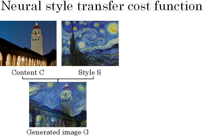
Remember what the problem formulation is. You're given a content image C, given a style image S and you goal is to generate a new image G.

In order to implement neural style transfer, what you're going to do is define a cost function J of G that measures how good is a particular generated image and we'll use gradient to descent to minimize J of G in order to generate this image.

How good is a particular image? Well, we're going to define two parts to this cost function. The first part is called the content cost. This is a function of the content image and of the generated image and what it does is it measures how similar is the contents of the generated image to the content of the content image C.

And then going to add that to a style cost function which is now a function of S,G and what this does is it measures how similar is the style of the image G to the style of the image S.

Finally, we'll weight these with two hyper parameters alpha and beta to specify the relative weighting between the content costs and the style cost.

It seems redundant to use two different hyper parameters to specify the relative cost of the weighting. One hyper parameter seems like it would be enough but the original authors of the Neural Style Transfer Algorithm, use two different hyper parameters.

I'm just going to follow their convention here.

The Neural Style Transfer Algorithm I'm going to present in the next few sections is due to Leon Gatys, Alexander Ecker and Matthias. Their papers is not too hard to read so after this sections if you wish, I certainly encourage you to take a look at their paper as well if you want.

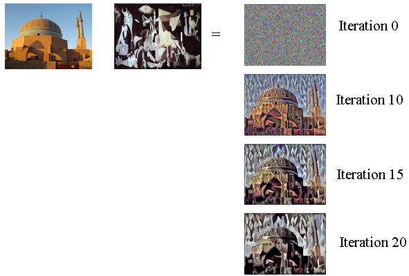
The way the algorithm would run is as follows, having to find the cost function J of G in order to actually generate a new image what you do is the following. You would initialize the generated image G randomly so it might be 100 by 100 by 3 or 500 by 500 by 3 or whatever dimension you want it to be.

Then we'll define the cost function J(G) then you can do is use gradient descent to minimize this so \( G = G - \frac{\partial J(G)}{\partial G}\)

In this process, you're actually updating the pixel values of this image G which is a 100 by 100 by 3 maybe RGB channel image.

Here's an example let's say you start with this content image and this style image. This is a another probably Picasso image.

Then when you initialize G randomly, you're initial randomly generated image is just this white noise image with each pixel value chosen at random.

As you run gradient descent, you minimize the cost function J of G slowly through the pixel value so then you get slowly an image that looks more and more like your content image rendered in the style of your style image.

In this section, you saw the overall outline of the Neural Style Transfer Algorithm where you define a cost function for the generated image G and minimize it.

Next, we need to see how to define the content cost function as well as the style cost function. Let's take a look at that starting in the next video.

The cost function of the neural style transfer algorithm had a content cost component and a style cost component.

Let's start by defining the content cost component.

Remember that this is the overall cost function of the neural style transfer algorithm. \( J(G) = \alpha J_{content} (C, G) + \beta J_{style} (S, G)\)

So, let's figure out what should the content cost function be. Let's say that you use hidden layer l to compute the content cost. If l is a very small number, if you use hidden layer one, then it will really force your generated image to pixel values very similar to your content image.

Whereas, if you use a very deep layer, then it's just asking, "Well, if there is a dog in your content image, then make sure there is a dog somewhere in your generated image. " So in practice, layer l chosen somewhere in between.

It's neither too shallow nor too deep in the neural network. And because you plan this yourself, in the programming exercise that you did at the end of this section, I'll leave you to gain some intuitions with the concrete examples in the exercise as well.

But usually, l' was chosen to be somewhere in the middle of the layers of the neural network, neither too shallow nor too deep. What you can do is then use a pre-trained ConvNet, maybe a VGG network, or could be some other neural network as well. And now, you want to measure, given a content image and given a generated image, how similar are they in content.

So let's let this \( a^{[l](C)} \) and \( a^{[l](G)} \) be the activations of layer l on these two images, on the images C and G.

So, if these two activations are similar, then that would seem to imply that both images have similar content. So, what we'll do is define \( J_{content} (C, G) \) as just how soon or how different are these two activations. \( J_{content} (C, G) = \frac{1}{2} || a^{[l](C)} - a^{[l](G)}||^2 \)

So, we'll take the element-wise difference between these hidden unit activations in layer l, between when you pass in the content image compared to when you pass in the generated image, and take that squared.

And you could have a normalization constant in front or not, so it's just one of the two or something else. It doesn't really matter since this can be adjusted as well by this hyperparameter alpha.

So, just be clear on using this notation as if both of these have been unrolled into vectors, so then, this becomes the square root of the l_2 norm between this and this, after you've unrolled them both into vectors.

There's really just the element-wise sum of squared differences between these two activation i.e. element-wise sum of squares of differences between the activations in layer l, between the images in C and G.

And so, when later you perform gradient descent on J(G) to try to find a value of G, so that the overall cost is low, this will incentivize the algorithm to find an image G, so that these hidden layer activations are similar to what you got for the content image.

So, that's how you define the content cost function for the neural style transfer. Next, let's move on to the style cost function.

In the last section, you saw how to define the content cost function for the neural style transfer.

Next, let's take a look at the style cost function.

So, what is the style of an image mean? Let's say you have an input image like shown below, they used to seeing a convnet like that, compute features that there's different layers. And let's say you've chosen some layer L, maybe that layer to define the measure of the style of an image.

What we need to do is define the style as the correlation between activations across different channels in this layer L activation.

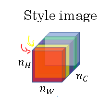
So here's what I mean by that. Let's say you take that layer L activation. So this is going to be nh by nw by nc block of activations, and we're going to ask how correlated are the activations across different channels.

So to explain what I mean by this may be slightly cryptic phrase, let's take a block of activations and let me shade the different channels by a different colors.

So in this below example, we have say five channels and which is why I have five shades of color here. In practice, of course, in neural network we usually have a lot more channels than five, but using just five makes it drawing easier.

But to capture the style of an image, what you're going to do is the following. Let's look at the first two channels. Let's see for the red channel and the yellow channel and say how correlated are activations in these first two channels.

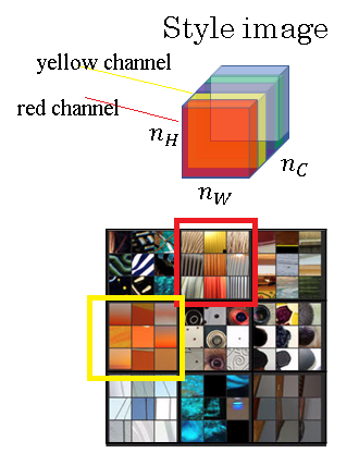
So, why does this capture style? Here's the 2D representation of the above 3D activation, in this the red channel and the yellow channel are shown using the red and yellow boxes.

This comes from again the paper by Matthew Zeiler and Rob Fergus that I have reference earlier. And let's say for the sake of arguments, that the red channel given above is trying to figure out if there's this little vertical texture in a particular position in the nh and let's say that this second channel, this yellow second channel corresponds to vaguely looking for orange colored patches.

What does it mean for these two channels to be highly correlated? Well, if they're highly correlated what that means is whatever part of the image has this type of subtle vertical texture, that part of the image will probably have these orange-ish tint.

And what does it mean for them to be uncorrelated? Well, it means that whenever there is this vertical texture, it's probably won't have that orange-ish tint.

And so the correlation tells you which of these high level texture components tend to occur or not occur together in part of an image and that's the degree of correlation that gives you one way of measuring how often these different high level features, such as vertical texture or this orange tint or other things as well, how often they occur and how often they occur together and don't occur together in different parts of an image.

And so, if we use the degree of correlation between channels as a measure of the style, then what you can do is measure the degree to which in your generated image, this first channel is correlated or uncorrelated with the second channel and that will tell you in the generated image how often this type of vertical texture occurs or doesn't occur with this orange-ish tint and this gives you a measure of how similar is the style of the generated image to the style of the input style image.

So let's now formalize this intuition. So what you can to do is given an image computes something called a style matrix, which will measure all those correlations we talks about on the last section.

So, more formally, let's let \( a^{[l]}_{i, j, k}\) denote the activation at position i,j,k in hidden layer l.

So i indexes into the height, j indexes into the width, and k indexes across the different channels.

So, in the previous section, we had five channels that k will index across those five channels. So what the style matrix will do is you're going to compute a matrix \( G^{[l]} \). This is going to be an nc by nc dimensional matrix, so it'd be a square matrix.

Remember you have nc channels and so you have an nc by nc dimensional matrix in order to measure how correlated each pair of them is.

So particular \( G^{[l]}_{k k'} \) will measure how correlated are the activations in channel k compared to the activations in channel k'.

Well here, k and k' will range from 1 through nc, the number of channels they're all up in that layer. So more formally, the way you compute \( G^{[l]}_{k k'} \) is by taking \( \sum_{i=1}^{{n_h}^{[l]}} \sum_{j=1}^{{n_w}^{[l]}} {a^{[l]}}_{ijk} {a^{[l]}}_{ijk'} \) .

So all this is doing is summing over the different positions that the image over the height and width and just multiplying the activations together of the channels k and k' prime' and that's the definition of \( G^{[l]}_{k k'} \). And you do this for every value of k and k' to compute this matrix G, also called the style matrix.

And so notice that if both of these activations tend to be lashed together, then \( G^{[l]}_{k k'} \) will be large, whereas if they are uncorrelated then \( G^{[l]}_{k k'} \) might be small.

And technically, I've been using the term correlation to convey intuition but this is actually the unnormalized cross of the areas because we're not subtracting out the mean and this is just multiplied by these elements directly. So this is how you compute the style of an image.

And you'd actually do this for both the style image s,n for the generated image G. So just to distinguish that this is the style image, maybe let me add a round bracket S there \( G^{[l](S)}_{k k'} \), just to denote that this is the style image for the image S and those are the activations on the image S.

And what you do is then compute the same thing for the generated image \( G^{[l](G)}_{k k'} \).

So, now, you have two matrices they capture what is the style with the image s and what is the style of the image G. And, by the way, we've been using the alphabet capital G to denote these matrices. In linear algebra, these are also called the gram matrix.

Finally, the cost function, the style cost function. If you're doing this on layer l between S and G, you can now define that to be just the difference between these two matrices

\( J(S, G) = \frac{1}{(2{n_h}^{[l]}{n_w}^{[l]}{n_c}^{[l]})^2} \sum_k \sum_{k'} (G^{[l](S)}_{k k'} - G^{[l](G)}_{k k'})^2 \)

. The authors actually used \( \frac{1}{(2{n_h}^{[l]}{n_w}^{[l]}{n_c}^{[l]})^2} \) for the normalization constants.

But a normalization constant doesn't matter that much because this causes multiplied by some hyperparameter b anyway.

So just to finish up, this is the style cost function defined using layer l and as you saw on the previous slide, this is basically the Frobenius norm between the two gram matrices computed on the image s and on the image G .

And, finally, it turns out that you get more visually pleasing results if you use the style cost function from multiple different layers.

So, the overall style cost function, you can define as sum over all the different layers of the style cost function for that layer.

\( J^{[l]}(S, G) = \frac{1}{(2{n_h}^{[l]}{n_w}^{[l]}{n_c}^{[l]})^2} \sum_k \sum_{k'} (G^{[l](S)}_{k k'} - G^{[l](G)}_{k k'})^2 \)

We should define the cost by some set of additional hyperparameters, which we'll denote as lambda l here. So what it does is allows you to use different layers in a neural network.

\( J_{style} (S, G) = \sum_l \lambda^{[l]} J_{style}^{[l]}(S, G) \)

And so just to wrap this up, you can now define the overall cost function as :

\( J(G) = \alpha J_{content} (C, G) + \beta J_{style} (S, G) \)

And if you do that, you can generate pretty good looking neural artistic and if you do that you'll be able to generate some pretty nice novel artwork.

So that's it for neural style transfer and I hope you have fun implementing it in this week's printing exercise.

Before wrapping up, there's just one last thing I want to share of you, which is how to do convolutions over 1D or 3D data rather than over only 2D images. Let's go into the last section.