We are now ready to see how to build one layer of a convolutional neural network, let's go through the example.

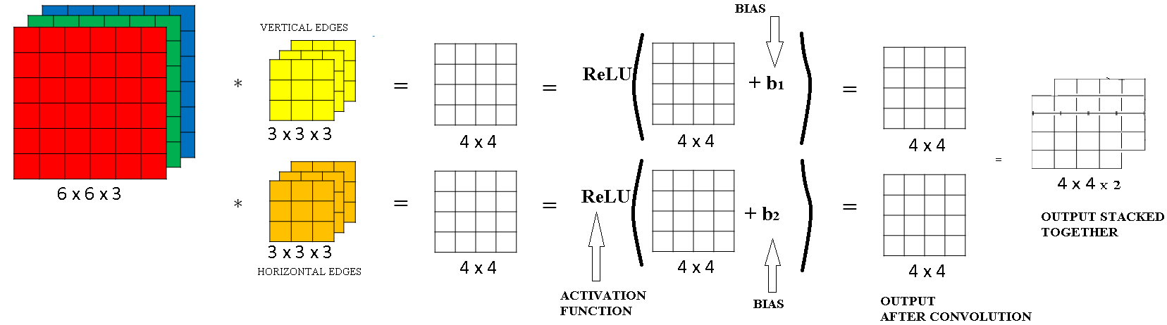
You've seen at the previous section how to take a 3D volume and convolve it with say two different filters.

In order to get in this example to different 4 by 4 outputs.

So let's say convolving with the first filter gives first 4 by 4 output, and convolving with this second filter gives a different 4 by 4 output. The final thing to turn this into a convolutional neural net layer, is that for each of these we're going to add it bias, so this is going to be a real number.

And with python broadcasting, you kind of have to add the same number so every one of these 16 elements. And then apply a non-linearity which for this illustration is ReLU non-linearity, and this gives you a 4 by 4 output. After applying the bias and the non-linearity.

And then for this thing at the bottom as well, you add some different bias, again, this is a real number. So you add the single number to all 16 numbers, and then apply some non-linearity, let's say a ReLU non-linearity. And this gives you a different 4 by 4 output.

Then same as we did before, if we take this and stack it up as follows, so we ends up with a 4 by 4 by 2 outputs. Then this computation where you come from a 6 by 6 by 3 to 4 by 4 by 2, this is one layer of a convolutional neural network.

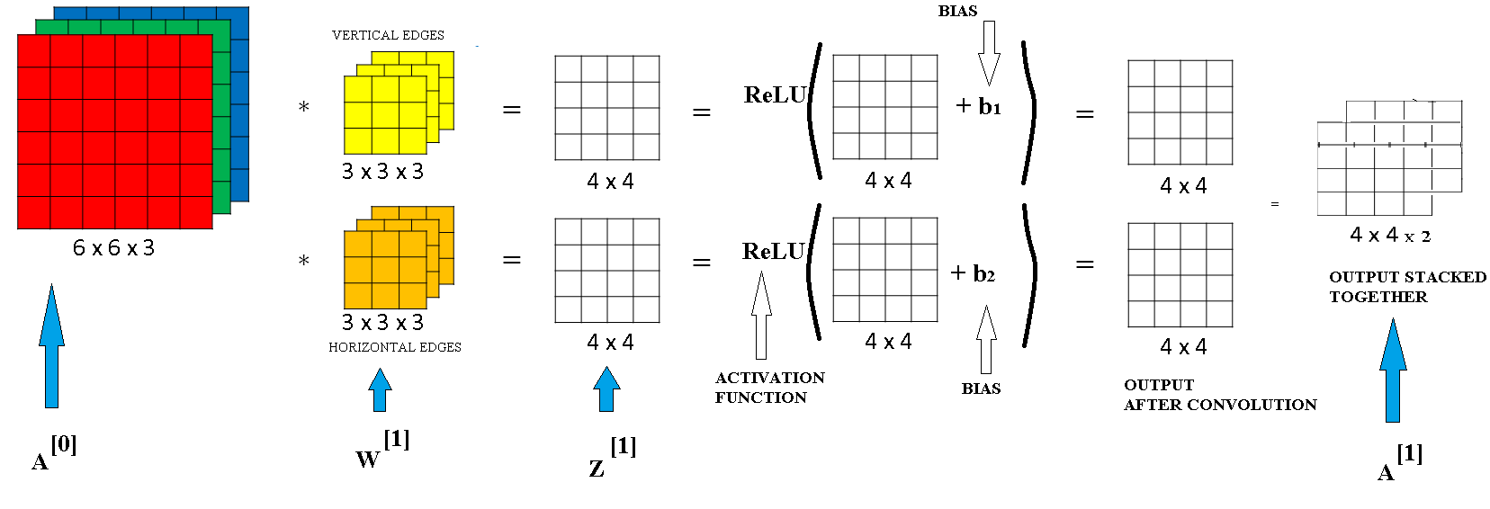
Remember that one step before the prop was something like \( a^{[0]} = x^{[0]}\\ z^{[1]} = w^{[1]}*x^{[0]} + b^{[1]}\\ a^{[1]} = g^{[1]}(z^{[1]})\\ . . . . z^{[L]} = w^{[L]}*x^{[L-1]} + b^{[L]}\\ a^{[L]} = g^{[L]}(z^{[L]})\\ \)

And the filters here, this plays a role similar to \(w^{[1]}\).

And you remember during the convolution operation, you were taking these 27 times 2 numbers (because you have two 3 x 3 x 3 filters so total 27 * 2 = 54 numbers) and multiplying them.

As seen from the below image a convolutional neural network takes an input image which has dimensions 6 x 6 x 3. This is \( A^{[0]} \). Then applies the two filters of dimensions 3 x 3 x 3. These are the weights of the first layer \( W^{[1]} \). Then it applies a bias to the output of the linear computation \( Z^{[1]} = W^{[1]} * A^{[0]} + b^{[1]} \). It then applies a non linear activation to the \( A^{[1]} = W^{[1]} A^{[0]} + b^{[1]} \).

Now in this example we have two filters, so we had two features of you will, which is why we wound up with our output 4 by 4 by 2.

But if for example we instead had 10 filters instead of 2, then we would have wound up with the 4 by 4 by 10 dimensional output volume. Because we'll be taking 10 of outputs not just two of them, and stacking them up to form a 4 by 4 by 10 output volume, and that's what \( A^{[1]} = W^{[1]} A^{[0]} + b^{[1]} \) would be.

So, to make sure you understand this, let's go through an exercise. Let's suppose you have 10 filters, not just two filters, that are 3 by 3 by 3 and 1 layer of a neural network, how many parameters does this layer have?

Well, let's figure this out. Each filter, is a 3 x 3 x 3 volume, so 3 x 3 x 3, so each filter has 27 parameters plus the bias so this gives you 28 parameters..

Now if you imagine that you actually have ten of these so that will be 280 parameters.

Notice one nice thing about this, is that no matter how big the input image is, the input image could be 1,000 by 1,000 or 5,000 by 5,000, but the number of parameters you have still remains fixed as 280. And you can use these ten filters to detect features, vertical edges, horizontal edges maybe other features anywhere even in a very, very large image is just a very small number of parameters.

So these is really one property of convolution neural network that makes less prone to overfitting then if you could. So once you've learned 10 feature detectors that work, you could apply this even to large images. And the number of parameters still is fixed and relatively small, as 280 in this example.

Let's just summarize the notation we are going to use to describe one layer to describe a covolutional layer in a convolutional neural network.

So layer l is a convolution layer, we are going to use \( f^{[l]} \) to denote the filter size. So previously we've been seeing the filters are f by f, and now this superscript square bracket l just denotes that this is a filter size of f by f filter layer l. And as usual the superscript square bracket l is the notation we're using to refer to particular layer l.

We are going to use \( p^{[l]} \) to denote the amount of padding. And again, the amount of padding can also be specified just by saying that you want a valid convolution, which means no padding, or a same convolution which means you choose the padding. So that the output size has the same height and width as the input size.

And then you're going to use \( s^{[l]} \) to denote the stride.

Now, the input to this layer are from the l-1 layer where \( {n_H}^{l-1} \) is the heights of the input image and \( {n_W}^{l-1} \) is the width of the input image and \( {n_C}^{l-1} \) is the number of filters of layer

To this we apply the filters which are the weights and get the output as \( {n_H}^{l} \) is the heights of the input image and \( {n_W}^{l} \) is the width of the input image and \( {n_C}^{l} \) is the number of filters of the layer.

If we use padding \( p^{[l]} \) and stride \( s^{[l]} \) at layer l then the final equation shall be: \( {n_W}^{l} = \left \lfloor \frac{{n_W}^{l-1} + 2p^{[l]} - f^{[l]}}{s^{[l]}} + 1 \right \rfloor \\ {n_H}^{l} = \left \lfloor \frac{{n_H}^{l-1} + 2p^{[l]} - f^{[l]}}{s^{[l]}} + 1 \right \rfloor \)

Then we obtain \( z^{[1]} \) with the dimensions as \( {n_W}^{l}, {n_H}^{l}, {n_C}^{l} \) to this we add the bias which has dimensions \( {n_C}^{l} \). Then we get the activation of layer l i.e. \( a^{[l]} \) this has the dimensions as \( {n_W}^{l}, {n_H}^{l}, {n_C}^{l} \).