In the last section, you saw how the Skip-Gram model allows you to construct a supervised learning task.

So we map from context to target and how that allows you to learn a useful word embedding.

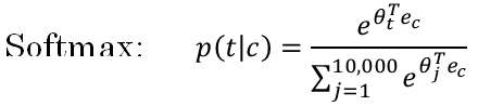
But the downside of that was the Softmax objective was slow to compute.

In this section, you'll see a modified learning problem called negative sampling that allows you to do something similar to the Skip-Gram model you saw just now, but with a much more efficient learning algorithm.

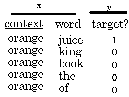
Let's see how you can do this. Most of the ideas presented in this section are due to Tomas Mikolov, Ilya Sutskever, Kai Chen, Greg Corrado, and Jeff Dean. So what we're going to do in this algorithm is create a new supervised learning problem. And the problem is, given a pair of words like orange and juice, we're going to predict, is this a context-target pair?

So in this example, orange juice was a positive example. And how about orange and king? Well, that's a negative example, so I'm going to write 0 for the target. So what we're going to do is we're actually going to sample a context and a target word.

So in this case, we have orange and juice and we'll associate that with a label of 1, so just put words in the middle. And then having generated a positive example, so the positive example is generated exactly how we generated it in the previous section. Sample a context word, look around a window of say, plus-minus ten words and pick a target word.

So that's how you generate the first row of this table with orange, juice, 1. And then to generate a negative example, you're going to take the same context word and then just pick a word at random from the dictionary.

So in this case, I chose the word king at random and we will label that as 0. And then let's take orange and let's pick another random word from the dictionary. Under the assumption that if we pick a random word, it probably won't be associated with the word orange, so orange, book, 0.

And let's pick a few others, orange, maybe just by chance, we'll pick the 0 and then orange. And then orange, and maybe just by chance, we'll pick the word of and we'll put a 0 there. And notice that all of these are labeled as 0 even though the word of actually appears next to orange as well.

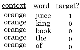
So to summarize, the way we generated this data set is, we'll pick a context word and then pick a target word and that is the first row of this table. That gives us a positive example. So context, target, and then give that a label of 1.

And then what we'll do is for some number of times say, k times, we're going to take the same context word and then pick random words from the dictionary, king, book, the, of, whatever comes out at random from the dictionary and label all those 0, and those will be our negative examples.

And it's okay if just by chance, one of those words we picked at random from the dictionary happens to appear in the window, in a plus-minus ten word window say, next to the context word, orange. Then we're going to create a supervised learning problem where the learning algorithm inputs x, inputs this pair of words, and it has to predict the target label to predict the output y.

So the problem is really given a pair of words like orange and juice, do you think they appear together? Do you think I got these two words by sampling two words close to each other? Or do you think I got them as one word from the text and one word chosen at random from the dictionary? It's really to try to distinguish between these two types of distributions from which you might sample a pair of words.

So this is how you generate the training set.

How do you choose k, Mikolov et al, recommend that maybe k is 5 to 20 for smaller data sets. And if you have a very large data set, then chose k to be smaller. So k equals 2 to 5 for larger data sets, and large values of k for smaller data sets. Okay, and in this example, I'll just use k = 4.

Next, let's describe the supervised learning model for learning a mapping from x to y. So here was the Softmax model you saw from the previous section.

And here is the training set we got from the previous section where again, this is going to be the new input x and this is going to be the value of y you're trying to predict.

So here we use c for the context word, target word as t, and output y to denote 0, 1, this is a context target pair. So what we're going to do is define a logistic regression model.

Say, that the chance of y = 1, given the input c, t pair \( P(y = 1| c, t) = \sigma({\theta_t}^T e_c) \)

So if you have k examples here, then you can think of this as having a k to 1 ratio of negative to positive examples. So for every positive examples, you have k negative examples with which to train this logistic regression-like model.

And so to draw this as a neural network, if the input word is orange, Which is word 6257, then what you do is, you input the one hop vector passing through E (embedding matrix) do the multiplication to get the embedding vector of word 6257.

And then what you have is really 10,000 possible logistic regression classification problems. Where one of these will be the classifier corresponding to, well, is the target word juice or not?

And then there will be other words, for example, there might be ones somewhere down here which is predicting, is the word king or not and so on, for these possible words in your vocabulary. So think of this as having 10,000 binary logistic regression classifiers, but instead of training all 10,000 of them on every iteration, we're only going to train five of them.

We're going to train the one responding to the actual target word we got and then train four randomly chosen negative examples. And this is for the case where k is equal to 4. So instead of having one giant 10,000 way Softmax, which is very expensive to compute, we've instead turned it into 10,000 binary classification problems, each of which is quite cheap to compute.

And on every iteration, we're only going to train five of them or more generally, k + 1 of them, of k negative examples and one positive examples. And this is why the computation cost of this algorithm is much lower because you're updating k + 1, let's just say units, k + 1 binary classification problems.

Which is relatively cheap to do on every iteration rather than updating a 10,000 way Softmax classifier. So you get to play with this algorithm in the programming exercise as well.

So this technique is called negative sampling because what you're doing is, you have a positive example, the orange and then juice. And then you will go and deliberately generate a bunch of negative examples, negative samplings, hence, the name negative sampling, with which to train four more of these binary classifiers.

And on every iteration, you choose four different random negative words with which to train your algorithm on. Now, before wrapping up, one more important detail with this algorithm is, how do you choose the negative examples? So after having chosen the context word orange, how do you sample these words to generate the negative examples?

So one thing you could do is sample the words in the middle, the candidate target words. One thing you could do is sample it according to the empirical frequency of words in your corpus. So just sample it according to how often different words appears. But the problem with that is that you end up with a very high representation of words like the, of, and, and so on.

One other extreme would be to say sample the negative examples uniformly at random, but that's also very non-representative of the distribution of English words. So the authors, Mikolov et al, reported that empirically, what they found to work best was to take a heuristic value, which is a little bit in between the two extremes of sampling from the empirical frequencies, meaning from whatever's the observed distribution in English text to the uniform distribution.

And so I'm not sure this is very theoretically justified, but multiple researchers are now using this heuristic, and it seems to work decently well.

So to summarize, you've seen how you can learn word vectors in a Softmax classier, but it's very computationally expensive. And in this section, you saw how by changing that to a bunch of binary classification problems, you can very efficiently learn words vectors.

And if you run this algorithm, you will be able to learn pretty good word vectors. Now of course, as is the case in other areas of deep learning as well, there are open source implementations. And there are also pre-trained word vectors that others have trained and released online under permissive licenses.

And so if you want to get going quickly on a NLP problem, it'd be reasonable to download someone else's word vectors and use that as a starting point. So that's it for the Skip-Gram model.

In the next section, I want to share with you yet another version of a word embedding learning algorithm that is maybe even simpler than what you've seen so far. So in the next section, let's learn about the Glove algorithm.