Colab

Imagine you have an extensive corpus of tweets that can be categorized as either positive or negative sentiment, but not both.

Within that corpus, the word happy is sometimes being labeled positive and sometimes negative.

One way to think about probabilities is by counting how frequently events occur.

Suppose you define event A as a tweets being labeled positive, then the probability of event A, shown as B of A , is calculated as the ratio between the counts of positive tweets in the corpus divided by the total number of tweets in the corpus.

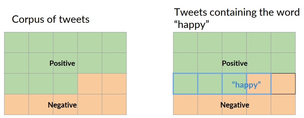
In this example, that number comes out to 13 over 20, or 0.65. You could also express this value as a percentage, 65 percent positive

A -> Positive tweet

P(A) = P(Positive) = Npos / N = 13 / 20 = 0.65

P(Negative) = 1 - P(Positive) = 0.35

. It's worth noting that the complimentary probability here, which is the probability of the tweets expressing a negative sentiment is just equal to one minus the probability of a positive sentiment.

Let's define Event B in a similar way by counting tweets containing the word happy. In this case, the total number of tweets containing the word happy, shown here as N-happy is 4.

B -> tweet contains happy .

P(B) = P(happy) = Nhappy / N

P(B) = 4 / 20 = 0.2

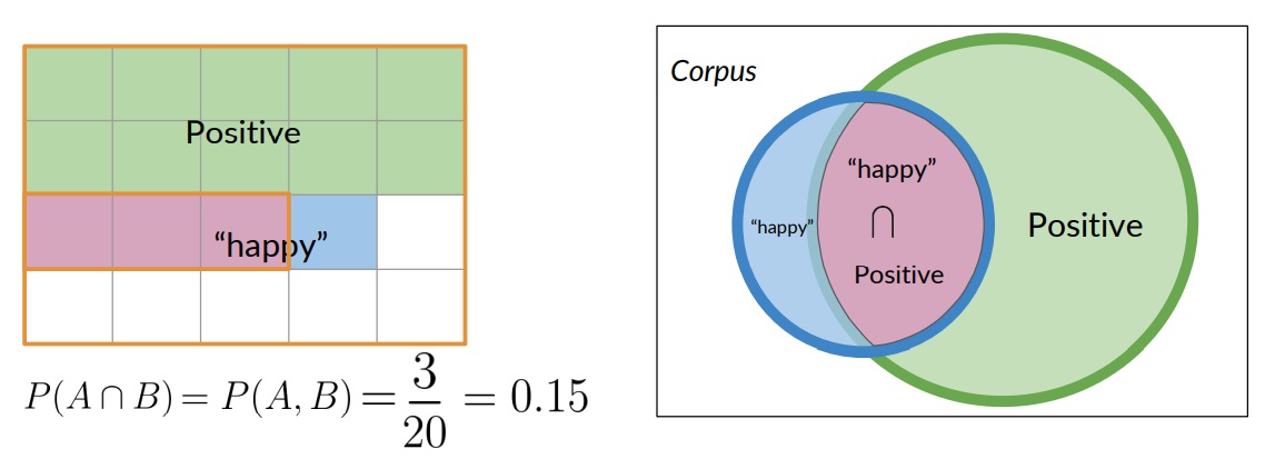
Take a look at the section of the diagram were tweets are labeled positive and also contain the word happy.

In the context of this diagram, the probability that a tweet is labeled positive and also contains the word happy is just the ratio of the area of the intersection divided by the area of the entire corpus.

In other words, if there were 20 tweets in the corpus, and three of them are labeled positive and also contain the word happy, then the associated probability is 3 divided by 20 or 0.15.

In order to derive Bayes rule, let's first take a look at the conditional probabilities.

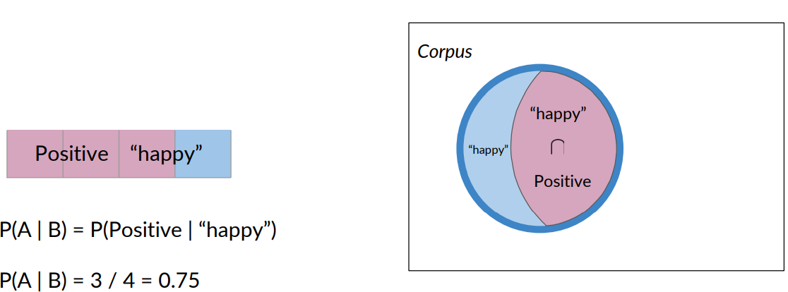
Now think about what happens if, instead of the entire corpus, you only consider tweets that contain the word happy.

This is the same as saying, given that a tweet contains the word happy with that, you would be considering only the tweets inside the blue circle, where many of the positive tweets are now excluded.

In this case, the probability that a tweet is positive, given that it contains the word happy, simply becomes the number of tweets that are positive and also contain the word happy.

We divide that by the number that contain the word happy. As you can see by this calculation, your tweet has a 75 percent likelihood of being positive if it contains the word happy.

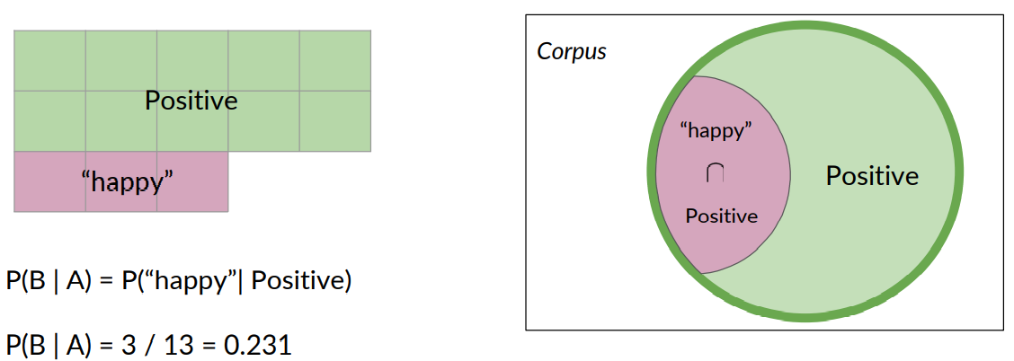
You could make the same case for positive tweets. The purple area denotes the probability that a positive tweet contains the word happy. In this case, the probability is 3 over 13, which is 0.231.

Conditional probabilities could be interpreted as the probability of an outcome B knowing that event A already happened, or given that I'm looking at an element from set A, the probability that it's also belongs to set B.

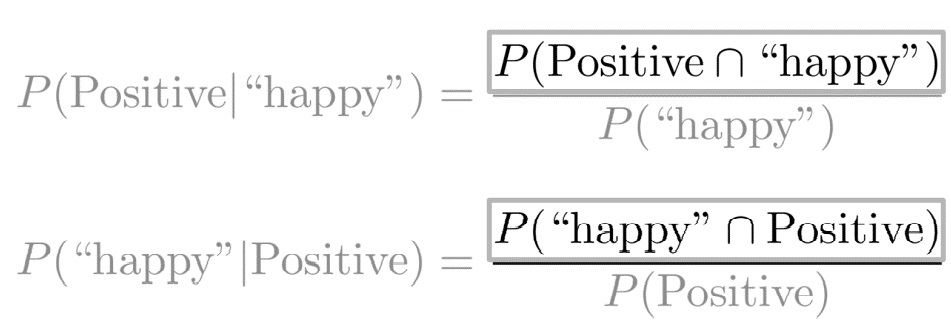
Using the previous example, the probability of a tweet being positive, given that it has the word happy, is equal to the probability of the intersection between the tweets that are positive and the tweets that have the word happy divided by the probability of a tweet given from the corpus having the word happy.

Now, you have the conditional probability of a tweet containing the word happy, given that it is a positive tweet.

Armed with both of these equations, you're now ready to derive Bayes rule.

To combine these equations, note that the intersection represents the same quantity, no matter which way it's written.

Knowing that, you can remove it from the equation, with a little algebraic manipulation, you are able to arrive at this equation. This is now an expression of Bayes rule in the context of the previous sentiment analysis problem.

More generally, Bayes rule states that the probability of x given y is equal to the probability of y given x times the ratio of the probability of x over the probability of y.

That's it. You just arrived at the basic formulation of Bayes rule, nicely done.

To wrap up, you just derive Bayes rule from expressions of conditional probability.

That's with Bayes rule, you can calculate the probability of x given y if you already know the probability of y given x and the ratio of the probabilities of x and y.

Naive Bayes is an example of supervised machine learning

It's called naive because this method makes the assumption that the features you're using for classification are all independent.

As before, you will begin with two corpora. One for the positive tweets and one for the negative tweets.

You need to extract the vocabulary or all the different words that appear in your corpus, along with their counts.

You get the word counts for each occurrence of a word in the positive corpus, then do the same for the negative corpus just like you did before.

Then you're going to get a total count of all the words in your positive corpus and do the same again for your negative corpus.

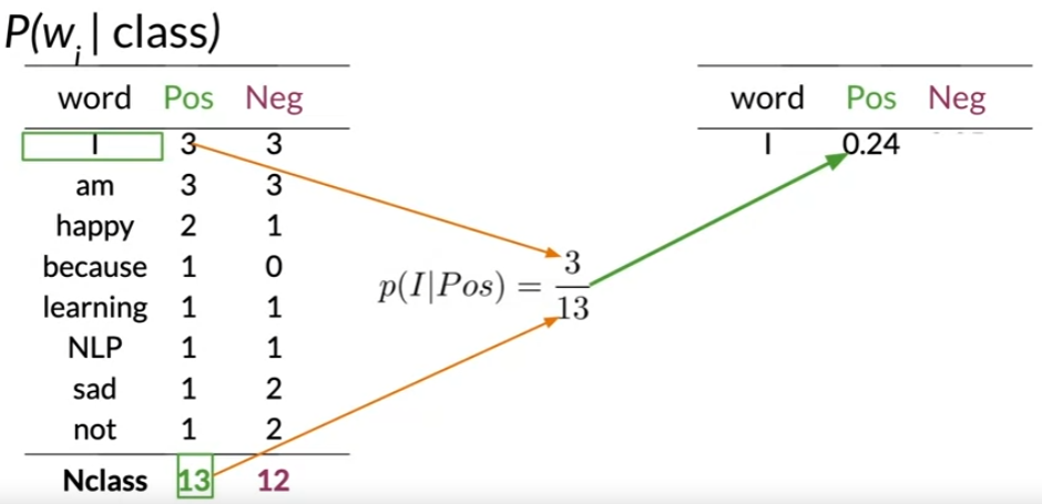
That is, you're just summing over the rows of this table. For positive tweets, there is a total of 13 words and for negative tweets, a total of 12 words.

This is the first new step for Naive Bayes and it's very important because it allows you to compute the conditional probabilities of each word given the class as you're about to see.

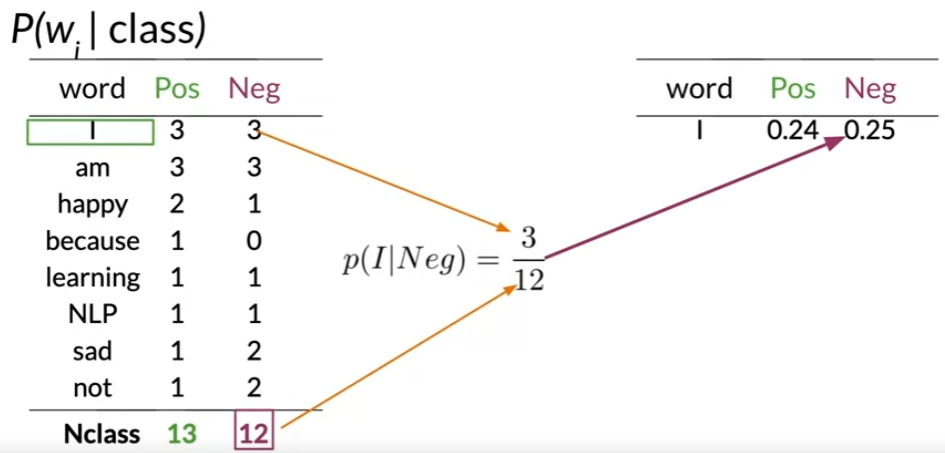
Now divide the frequency of each word in a class by it's corresponding sum of words in the class.

For the word I, the conditional probability for the positive class would be 3//13. You store that value in a new table with the corresponding value, 0.24. Now for the word I in the negative class, you get 3/12. You store that in your new table with the corresponding value, 0.25.

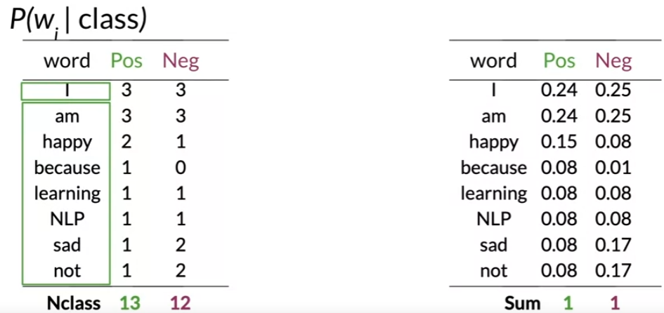
Now apply the same procedure for each word in your vocabulary to complete the table of conditional probabilities.

One key property of this table is that if you sum over all the probabilities for each class, you will get 1.

Let's investigate this table further to see what these numbers mean.

First, note how many words have a nearly identical conditional probability, like I'm learning and then NLP. The interesting thing here is words that are equally probable don't add anything to the sentiment.

In contrast to these neutral words, look at some of these other words like happy, sad, and not.

They have a significant difference between probabilities.

These are your power words tending to express one sentiment or the other. These words carry a lot of weight in determining your tweet sentiments.

Now let's take a look at because. As you can see, it only appears in the positive corpus.

It's conditional probability for the negative class is 0.

When this happens, you have no way of comparing between the two corpora, which will become a problem for your calculations.

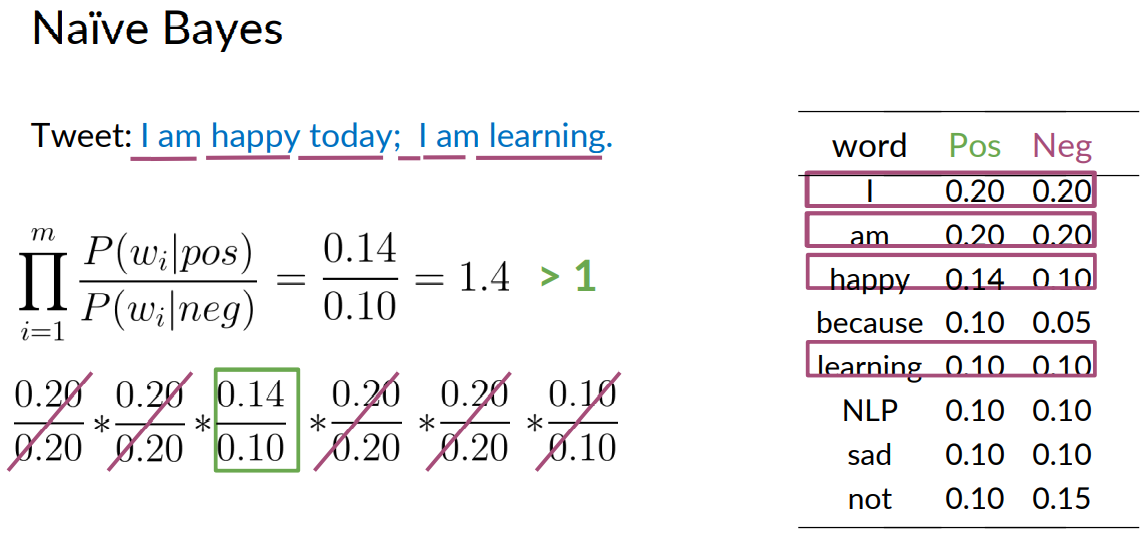
To avoid this, you will smooth your probability function. Say you get a new tweet from one of your friends and the tweet says, "I'm happy today, I'm learning." You want to use the table of probabilities to predict the sentiments of the whole tweet.

This expression is called the Naive Bayes inference condition rule for binary classification.

This expression says that you're going to take the product across all of the words in your tweets of the probability for each word in the positive class divide it by the probability in the negative class.

Let's calculate this product for this tweet. For each word, select it's probabilities from the table.

For I, you get a positive probability of 0.2 and a negative probability of 0.2.

The ratio that goes into the product is just 0.2/0.2. For I'm, you also get 0.2/0.2.

For happy, you get 0.14/0.10.

For today, you don't find any word in the table, meaning this word is not in your vocabulary. So you won't include any term in the score.

For the second occurrence of I again, you'll have 0.2/0.2. For the second occurrence of I'm, you'll have 0.2/0.2 and learning gets 0.10/0.10.

Now note that's all the neutral words in the tweet, like I and I'm, just cancel out in the expression. What you end up is with 0.14/ 0.10, which is equal to 1.4.

This value is higher than one, which means that overall, the words in the tweets are more likely to correspond to a positive sentiment.

So you conclude that the tweet is positive.

So far, you've created a table to store the conditional probabilities of words in your vocabulary and applied the Naive Bayes inference condition rule for binary classification of a tweet.

We usually compute the probability of a word given a class as follows:

\( P\left(\mathrm{w}_{\mathrm{i}} \mid \text { class }\right)=\frac{\text { freq }\left(\mathrm{w}_{\mathrm{i}}, \text { class }\right)}{\mathrm{N}_{\text {class }}} \quad \text { class } \in\{\text { Positive, Negative }\} \)

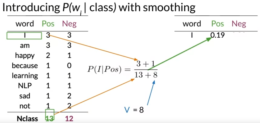
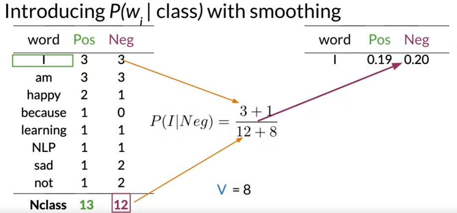
However, if a word does not appear in the training, then it automatically gets a probability of 0, to fix this we add smoothing as follows

\( P\left(\mathrm{w}_{\mathrm{i}} \mid \mathrm{class}\right)=\frac{freq\left(\mathrm{w}_{\mathrm{i}}, \text{class}\right)+1}{\left(\mathrm{N}_{\text {class }}+\mathrm{V}\right)} \)

Note that we added a 11 in the numerator, and since there are V words to normalize, we add V in the denominator.

\(N_{class}\) : frequency of all words in class

V: number of unique words in vocabulary

Recall previously a table was created with each word and its occurance in positive tweets and negative tweets.

Then we calculated the P(word|Pos) which is the probability of the a positive tweet having the word in it and P(word|Neg) which is probability of the negative tweet having the word in it.

\( P\left(\mathrm{w}_{\mathrm{i}} \mid \text { class }\right)=\frac{\text { freq }\left(\mathrm{w}_{\mathrm{i}}, \text { class }\right)}{\mathrm{N}_{\text {class }}} \quad \text { class } \in\{\text { Positive, Negative }\} \)

Then with laplacian smoothing this ratio changed to

\( P\left(\mathrm{w}_{\mathrm{i}} \mid \mathrm{class}\right)=\frac{freq\left(\mathrm{w}_{\mathrm{i}}, \text{class}\right)+1}{\left(\mathrm{N}_{\text {class }}+\mathrm{V}\right)} \)

Then we use naive bayes rule

To do inference, you can compute the following:

\( \frac{P(p o s)}{P(n e g)} \prod_{i=1}^{m} \frac{P\left(w_{i} \mid p o s\right)}{P\left(w_{i} \mid n e g\right)} \)

As m gets larger, we can get numerical flow issues, so we introduce the log, which gives you the following equation:

\( \log \left(\frac{P(p o s)}{P(n e g)} \prod_{i=1}^{n} \frac{P\left(w_{i} \mid p o s\right)}{P\left(w_{i} \mid n e g\right)}\right) \Rightarrow \log \frac{P(p o s)}{P(n e g)}+\sum_{i=1}^{n} \log \frac{P\left(w_{i} \mid p o s\right)}{P\left(w_{i} \mid n e g\right)} \)

The first component is called the log prior and the second component is the log likelihood. We further introduce \lambda λ as follows

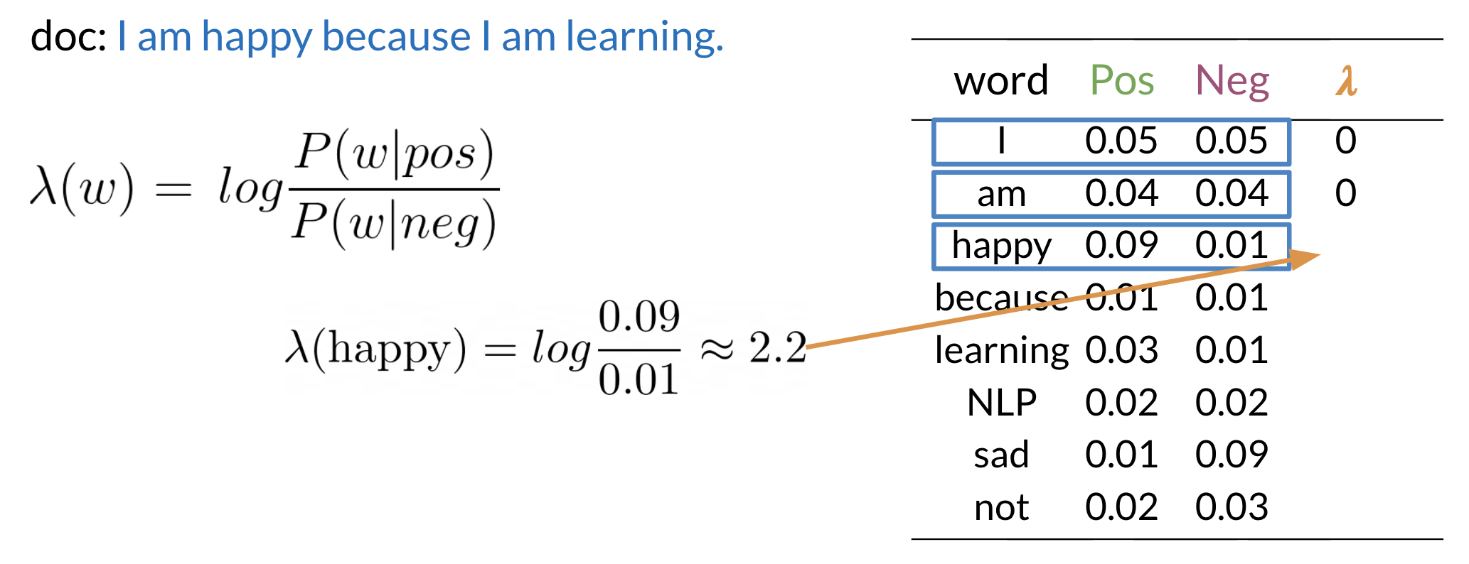
Once you computed the λ dictionary, it becomes straightforward to do inference:

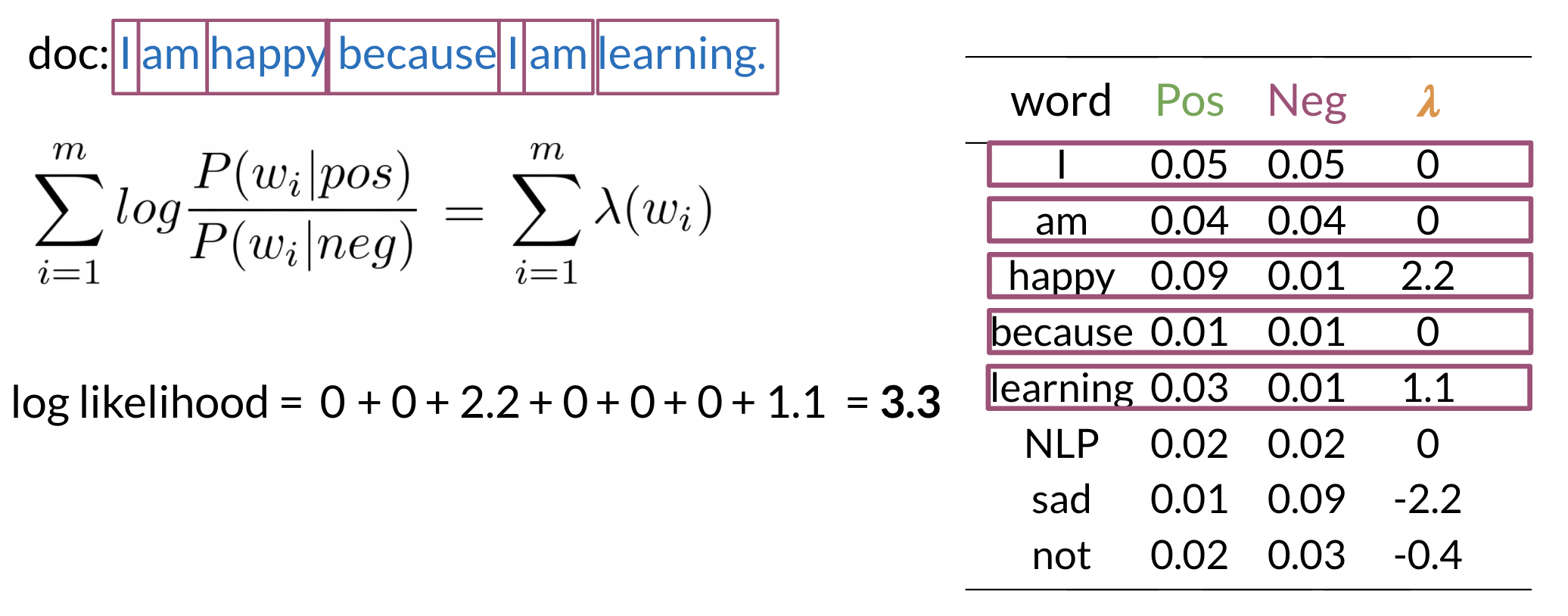
As you can see above, since 3.3 > 0 , we will classify the document to be positive. If we got a negative number we would have classified it to the negative class.