You've already learned about the basic structure of an RNN.

In this section, you'll see how backpropagation in a recurrent neural network works.

As usual, when you implement this in one of the programming frameworks, often, the programming framework will automatically take care of backpropagation.

But I think it's still useful to have a rough sense of how backprop works in RNNs.

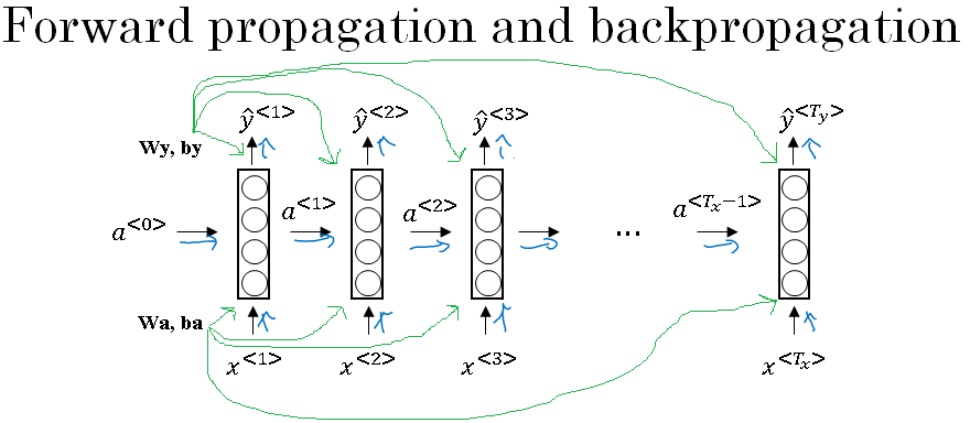
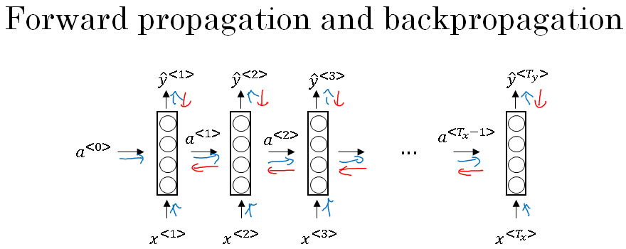
Let's take a look. You've seen how, for forward prop, you would computes the activations from left to right as follows in the neural network, and so you've outputs all of the predictions. This calculation is shown in blue arrows below.

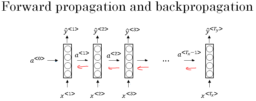
In backprop, as you might already have guessed, you end up carrying backpropagation calculations in basically the opposite direction of the forward prop arrows.

So, let's go through the forward propagation calculation. You're given this input sequence \(X^{<1>}, X^{<2>}, X^{<3>}, ... , X^{Tx} \).

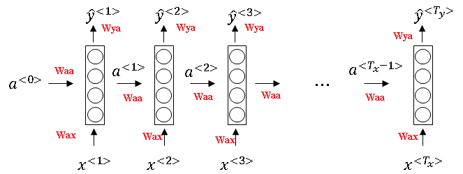
And then using \(X^{<1>}\) and say, \(A^{<0>} \), you're going to compute the activation, times that one, and then together, \( X^{<2>} \) together with \(A^{<1>} \) are used to compute \(A^{<2>} \), and then \(A^{<3>} \), and so on, up to \(A^{Tx} \).

And then to actually compute \(A^{<1>} \), you also need the parameters.

We'll just draw this below, W_a and b_a, those are the parameters that are used to compute \(A^{<1>} \).

And then, these parameters are actually used for every single timestep so, these parameters are actually used to compute \(A^{<2>} , A^{<3>} \) and so on, all the activations up to last timestep depend on the parameters W_a and b_a.

In the figure above, given \(A^{<1>}\) your neural network can then compute the first prediction, \(\hat{y}^{<1>}\), and then the second timestep, \(\hat{y}^{<2>}\) , \(\hat{y}^{<3>}\), and so on, with\(\hat{y}^{Ty}\).

So, to compute \(\hat{y}\), you need the parameters, W_y as well as b_y, and this goes into the nodes as shown below.

Next, in order to compute backpropagation, you need a loss function.

So let's define an element-wise loss function, which is supposed for a certain word in the sequence.

\( L^{t}(y^{t},\hat{y}^{t}) = -y^{t}log(\hat{y}^{t}) - (1 - y^{t})log(1 - \hat{y}^{t}) \)

\( y^{t},\hat{y}^{t} \) are the expected output and the actual output.

So I'm going to define this as the standard logistic regression loss, also called the cross entropy loss.

This may look familiar to you from where we were previously looking at binary classification problems.

So this is the loss associated with a single prediction at a single position or at a single time set, t, for a single word.

Let's now define the overall loss of the entire sequence, so L will be defined as the sum overall t equals one to, i guess, T_x.

\( L(y^{t},\hat{y}^{t}) = \sum_{t = 1}^{Ty} L^{t}(y^{t},\hat{y}^{t}) \)

T_x is equals to T_y in this example of the losses for the individual timesteps, comma y^<t>.

And then, so, just have to L without this superscript T.

This is the loss for the entire sequence. So, in a computation graph, to compute the loss given \( \hat{y}^{<1>} \) you can then compute the loss for the first timestep given that you compute the loss for the second timestep, the loss for the third timestep, and so on, the loss for the final timestep.

And then lastly, to compute the overall loss, we will take these and sum them all up to compute the final L using that equation, which is the sum of the individual per timestep losses.

So, this is the computation problem and from the earlier examples you've seen of backpropagation, it shouldn't surprise you that backprop then just requires doing computations or parsing messages in the opposite directions.

So, all of the four propagation steps arrows, so you end up doing that. And that then, allows you to compute all the appropriate quantities that lets you then, take the derivatives, and update the parameters using gradient descent.

Now, in this back propagation procedure, the most significant message or the most significant recursive calculation is the one given below, which goes from right to left, and that's why it gives this algorithm a pretty fast name called backpropagation through time.

And the motivation for this name is that for forward prop, you are scanning from left to right, increasing indices of the time, t, whereas, the backpropagation, you're going from right to left, you're kind of going backwards in time.

So, I hope that gives you a sense of how forward prop and backprop in RNN works.

Now, so far, you've only seen this main motivating example in RNN, in which the length of the input sequence was equal to the length of the output sequence.

In the next section, I want to show you a much wider range of RNN architecture, so I'll let you tackle a much wider set of applications. Let's go on to the next section.