Mean and Variance of a Random Variable: Introduction
In the Exploratory Data Analysis (EDA) section, we displayed the distribution of one quantitative variable with a histogram, and supplemented it with numerical measures of center and spread. We are doing the same thing here. We display the probability distribution of a discrete random variable with a table, formula or histogram, and supplement it with numerical measures of the center and spread of the probability distribution. These measures are the mean and standard deviation of the random variable.
Let's begin by revisiting an example we saw in EDA.
World Cup Soccer Recall that we used the following data from 3 World Cup tournaments (a total of 192 games) to introduce the idea of a weighted average. We've added a third column to our table that gives us relative frequencies.
total # goals/game frequency relative frequency 0 17 17 / 192 = 0.089 1 45 45 / 192 = 0.234 2 51 51 / 192 = 0.266 3 37 37 / 192 = 0.193 4 25 25 / 192 = 0.130 5 11 11 / 192 = 0.057 6 3 3 / 192 = 0.016 7 2 2 / 192 = 0.010 8 1 1 / 192 = 0.005 the mean for this data is: \( \frac{0*17 + 1*45 + 2*51 + 3*37 + 4*25 + 5*11 + 6*3 + 7*2 + 8*1}{192} \)
distributing the division by 192 we get: \( 0*(17/192) + 1*(45/192) + 2*(51/192) + 3*(37/192) + 4*(25/192) + 5*(11/192) + 6*(3/192) + 7*(2/192) + 8*(1/192) \)
Notice that the mean is each number of goals per game multiplied by its relative frequency. Since we usually write the relative frequencies as decimals, we can see that:
mean number of goals per game = 0(0.089) + 1(0.234) + 2(0.266) + 3(0.193) + 4(0.130) + 5(0.057) + 6(0.016) + 7(0.010) + 8(0.005)
mean number of goals per game = 2.36, rounded to two decimal places
Mean of a Random Variable : In Exploratory Data Analysis, we used the mean of a sample of quantitative values—their arithmetic average—to tell the center of their distribution. We also saw how a weighted mean was used when we had a frequency table. These frequencies can be changed to relative frequencies.
So we are essentially using the relative frequency approach to find probabilities. We can use this to find the mean, or center, of a probability distribution for a random variable by reporting its mean, which will be a weighted average of its values; the more probable a value is, the more weight it gets.
As always, it is important to distinguish between a concrete sample of observed values for a variable versus an abstract population of all values taken by a random variable in the long run.
Whereas we denoted the mean of a sample as \( \overline{x} \), we now denote the mean of a random variable as \( \mu_x \). Let's see how this is done by looking at a specific example.
Example: Xavier's Production Line
Xavier's production line produces a variable number of defective parts in an hour, with probabilities shown in this table:
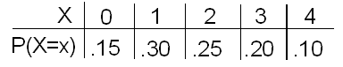 How many defective parts are typically produced in an hour on Xavier's production line? If we sum up the possible values of X, each weighted with its probability, we have
\( \mu_x = 0(0.15) + 1(0.3) + 2(0.25) + 3(0.2) + 4(0.1) = 1.8 \)
Mean of a discrete random variable : (definition) In general, for any discrete random variable X with probability distribution
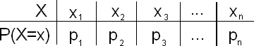
the mean of X is defined to be \( \mu_x = x_1p_1 + x_2p_2 + x_3p_3 .. + x_np_n = \sum_{i=1}^{n} x_ip_i \)
In general, the mean of a random variable tells us its "long-run" average value. It is sometimes referred to as the expected value of the random variable. But this expression may be somewhat misleading, because in many cases it is impossible for a random variable to actually equal its expected value.
For example, the mean number of goals for a World Cup soccer game is 2.36. But we can never expect any single game to result in 2.36 goals, since it is not possible to score a fraction of a goal.
Rather, 2.36 is the long-run average of all World Cup soccer games. In the case of Xavier's production line, the mean number of defective parts produced in an hour is 1.8. But the actual number of defective parts produced in any given hour can never equal 1.8, since it must take whole number values.
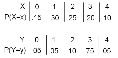
Example: Xavier's and Yves' Production Lines
Recall the probability distribution of the random variable X, representing the number of defective parts in an hour produced by Xavier's production line.
The number of defective parts produced each hour by Yves' production line is a random variable Y with the following probability distribution:
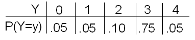
Look at both probability distributions. Both X and Y take the same possible values (0, 1, 2, 3, 4). However, they are very different in the way the probability is distributed among these values.
- Explanation :
Indeed, the probability distribution of Y has most of the weight (80%) on the larger values (3, 4), while the distribution of X has most of the weight (70%) on the smaller values (0, 1, 2). Since the mean is an average of the values weighted by their probabilities, we would expect the mean of Y to be larger than the mean of X, which is 1.8.
- Explanation :
Indeed, the mean of Y is 0(.05) + 1(.05) + 2(.10) + 3(.75) + 4(.05) = 2.7.
Applications of the Mean : Example: Pizza Delivery #1
Means of random variables are useful for telling us about long-run gains in sales, or for insurance companies.
Your favorite pizza place delivers only one kind of pizza, which is sold for Rs. 10, and costs the pizza place Rs. 6 to make. The pizza place has the following policy regarding delivery: if the pizza takes longer than half an hour to arrive, there is no charge.
Let the random variable X be the pizza place's gain for any one pizza.
Experience has shown that delivery takes longer than half an hour only 10 percent of the time.
Find the mean gain per pizza, \( \mu_x \).
In order to find the mean of X, we first need to establish its probability distribution—the possible values and their probabilities.
The random variable X has two possible values: either the pizza costs them $6 to make and they sell it for Rs. 10, in which case X takes the value Rs. 10 - Rs. 6 = Rs. 4, or it costs them Rs. 6 to make and they give it away, in which case X takes the value Rs. 0 - $6 = -$6. The probability of the latter case is given to be 10 percent, or .1, so using complements, the former has probability .9. Here, then is the probability distribution of X: \( \mu_x = 4*.9 + -6*.1 = 3 \)
In the long run, the pizza place gains an average of Rs. 3 per pizza delivered.
Example: Pizza Delivery #2
If the pizza place wants to increase its mean gain per pizza to $3.90, how much should it raise the price from $10? We need to replace the original cost of 10 with an as-yet-to-be-determined new cost N, resulting in this probability distribution table:
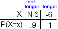
Next, setting \( \mu_x \) equal to +3.90 instead of +3, we solve
3.9 = (N-6)*.9 + -6*.1 = .9N - 6 OR .9N = 9.9
Therefore, the new price must be 11 dollars.
Scenario: Shipping Rates
The Acme Shipping Company has learned from experience that it costs $14.80 to deliver a small package overnight. The company charges $20 for such a shipment, but guarantees that they will refund the $20 charge if it does not arrive within 24 hours. Let X be a discrete random variable representing the outcomes for the Acme Shipping Company. What are the possible values for X?
Answer : If the package is delivered within 24 hours, the net amount the company gets is the fee they charge minus their cost, or 20 - 14.80 = 5.20. If the package is not delivered within 24 hours, they must return the fee. So the net amount the company gets is 20 - 20 - 14.80 = -14.80.
Suppose Acme successfully delivers 96% of its packages within 24 hours. What are the probabilities that correspond to the values for X you found in the previous question?
Answer : Since they deliver within 24 hours with a probability of 0.96, 0.96 corresponds to 5.20. Not delivering within 24 hours is the complement of delivering within 24 hours. Thus, the probability corresponding to -14.80 is 1 - 0.96 = 0.04.
Using the information from the previous two questions, what is the expected gain or loss for delivering a package?
Answer : μX = (5.20)(0.96) + (-14.80)(0.04) = 4.40. This means that in the long run, each package delivered has an expected gain of $4.40
Example: Raffle
In order to raise money, a charity decides to raffle off some prizes. The charity sells 2,000 raffle tickets for $5 each. The prizes are:
10 movie packages (two tickets plus popcorn) worth $25 each
5 dinners for two worth $50 each
2 smart phones worth $200 each
1 flat-screen TV worth $1,500What is the expected gain or loss if you buy a single raffle ticket? The expected value can be written as E(X).
There are 5 possible outcomes when you buy a ticket: win movie package, win dinner for two, win smart phone, win TV, win nothing.
prize net gain or loss probability movie package 25 - 5 10 / 2000 dinner for two 50 - 5 5 / 2000 smart phone 200 - 5 2 / 2000 TV 1500 - 5 1 / 2000 nothing 0 - 5 (2000 - 10 - 5 - 2 - 1) / 2000 The previous information is summarized below in a probability distribution:
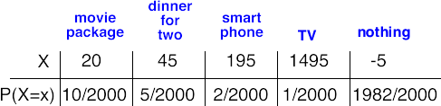
\( \mu_x = E(X) = 20*\frac{10}{2000} + 45*\frac{5}{2000} + 195*\frac{2}{2000} + 1495*\frac{1}{2000} + -5*\frac{1982}{2000} \)
\( E(X) = \frac{-7600}{2000} = -3.8 \)
Since we got a negative number, we have an expected loss of $3.80 for each raffle ticket purchased. Recall that this is based upon a long-run average.
Each raffle ticket has only 5 possible outcomes:
$20 net gain if you win the movie package
$45 net gain if you win the dinner for two
$195 net gain if you win the smart phone
$1,495 net gain if you win the TV
$5 net loss if you do not win a prize
It should not be surprising that you have an expected loss. After all, the charity's goal is to raise money. If you have an expected loss of $3.80 per ticket, they will have an expected gain of $3.80 per ticket. Each ticket gives the charity +5 (it was -5 for you). The prizes are reversed, too. For example, the movie package is -20 + 5 for the charity (it was 20 - 5 for you).
Mean of a Random Variable: Examples - Life Insurance #1
Suppose you work for an insurance company, and you sell a $100,000 whole-life insurance policy at an annual premium of Rs. 1,200. (This means that the person who bought this policy pays Rs. 1,200 per year so that in the event that he or she dies, the policy beneficiaries will get Rs. 100,000). Actuarial tables show that the probability of death during the next year for a person of your customer's age, sex, health, etc. is .005. Let the random variable X be the company's gain from such a policy.
What is the expected or mean gain (amount of money made by the company) for a policy of this type?
In other words, we need to find \( \mu_x \) .
Since this is a whole-life policy, there are two possibilities here; either the customer dies this year (which you are given will happen with probability 0.005), or the customer does not die this year (which, by the complement rule, must be 0.995).
In both cases, the company gets the Rs. 1,200 premium. If the customer lives, the company just gains the Rs. 1,200, but if the customer dies, the company needs to pay Rs. 100,000 to the customer's beneficiaries. Therefore, here is the probability distribution of X:
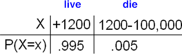
Their average, or expected, gain overall is
\( \mu_x \) = 1200(0.995) + (1200 - 100,000)(0.005) = Rs. 700 .
Example: Life Insurance #2
Suppose that five years have passed and your actuarial tables indicate that the probability of death during the next year for a person of your customer's current age has gone up to 0.0075. Obviously, this change in probability should be reflected in the annual premium (since it is slightly more risky for the insurance company to insure the customer).
What should the annual premium be (instead of Rs. 1,200) if the company wants to keep the same expected gain?
Now we substitute 0.0075 for 0.005, replace 1,200 with an unknown new premium N, and set the mean gain equal to 700, as it was before:
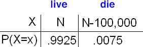
We need to solve:
700 = (N)(0.9925) + (N - 100,000)(0.0075)
Using some algebra:
700 = N - 750
Finally : N = 1450In order to keep the same expected gain of Rs.700, the company should increase that customer's premium to Rs. 1,450.
Scenario: Fire Insurance
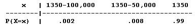
Suppose that you work for an insurance company and you sell a Rs.100,000 fire insurance policy at an annual premium of Rs.1,350. Experience has shown that:
The probability of total loss (due to fire) to a house in that area and of the size of your customer's house is .002 (in which case the insurance company will pay the full Rs.100,000 to the customer).
The probability of 50% damage (due to fire) to a house in that area and of the size of your customer's house is .008 (in which case the insurance company will pay only Rs.50,000 to the customer).
Let the random variable X be the insurance company's annual gain from such a policy (i.e., the amount of money made by the insurance company from such a policy).
Q. Find the probability distribution of X. In other words, list the possible values that X can have, and their corresponding probabilities. (Hint: There are three possibilities here: no fire, total loss due to fire, 50% damage due to fire).
There are three possibilities that correspond to the three possible values of X in this example. In every case, the insurance company is gaining the amount of the policy cost, which is Rs.1,350.
If there is total loss due to fire (which happens with probability .002), the insurance company has to pay the customer $100,000, and therefore the company's gain is: Rs.1,350 - Rs.100,000.
If there is 50% damage due to fire (which happens with probability .008), the insurance company has to pay the customer $50,000, and therefore the company's gain is: Rs.1,350 - Rs.50,000.
If there is no fire (which must happen with the "remaining probability" of 1 - .002 - .008 = .99), the insurance company has to pay nothing, and so is left with the premium gain of Rs. 1,350.
To summarize, the probability distribution of X is:
Q. What is the mean (expected) annual gain for a policy of this type? In other words, what is the mean of X?
Using the definition of the mean of a discrete random variable, we will average the possible values weighted by their corresponding probabilities.
Mean of X = (1,350 - 100,000)(.002) + (1,350 - 50,000)(.008) + 1,350(.99) = 750.
The expected gain of such a policy is Rs. 750. Since the insurance company probably sells a lot of policies of this type, in the majority of them (99%) the company will gain money (Rs. 1,350), and in the remaining 1% of them, it will lose (either 1,350 - 100,000 or 1,350 - 5,0000). Averaging over all such policies, the company is going to make about Rs. 750 from each such fire insurance policy.
Q. The insurance company gets information about gas leakage in several houses that use the same gas provider that your customer does. In light of this new information, the probabilities of total loss and 50% damage (that were originally 0.002 and 0.008, respectively) are tripled (to 0.006 for total loss and 0.024 for 50% damage). Obviously, this change in the probabilities should be reflected in the annual premium, to account for the added risk that the insurance company is taking. What should be the new annual premium (instead of Rs. 1,350), if the company wants to keep its expected gain of Rs. 750?
Guidance: Let the new premium (instead of 1,350) be denoted by N, for new. Set up the new probability distribution of X using the updated probabilities, and using N instead of 1,350. (The answer to question 1 will help.)
The question now is: What should the value of N (the new premium) be, if we want the mean of X to remain 750?
Set up an equation with N as unknown, and solve for N.
Here is the new probability distribution of X:
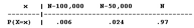
Note that we updated the probabilities of total loss and 50% damage by tripling them, and the probability of no fire has changed to 1 - 0.006 - 0.024 = 0.97. The company wants to keep the same annual gain from the policy ($750), and the question is, what should the new premium (N) be that will satisfy this? In other words, we need to solve the following equation for N:
750 = (N - 100,000)(0.006) + (N - 50,000)(0.024) + N(0.97)
Thus, 750 = N - 600 - 1,200, or N - 1,800.
And therefore, N = 750 + 1,800 = 2,550.
In order to account for the added risk that the insurance company is taking by continuing to insure the customer, the premium changes from Rs. 1,350 to Rs. 2,550.
Variance and Standard Deviation of a Discrete Random Variable
In Exploratory Data Analysis, we used the mean of a sample of quantitative values (their arithmetic average, \( \overline{x} \) ) to tell the center of their distribution, and the standard deviation(s) to tell the typical distance of sample values from their mean.
We described the center of a probability distribution for a random variable by reporting its mean \( \mu_x \), and now we would like to establish an accompanying measure of spread.
Our measure of spread will still report the typical distance of values from their means, but in order to distinguish the spread of a population of all of a random variable's values from the spread (s) of sample values
We will denote the standard deviation of the random variable X with the Greek lower case "σ," and use a subscript to remind us what is the variable of interest (there may be more than one in later problems):
Notation: \( \sigma_x \) We will also focus more frequently than before on the squared standard deviation, called the variance, because some important rules we need to invoke are in terms of variance \( \sigma^2_x \) rather than standard deviation \( \sigma_x \) .
Example: Xavier's Production Line
Recall that the number of defective parts produced each hour by Xavier's production line is a random variable X with the following probability distribution:
-
We found the mean number of defective parts produced per hour to be \( \mu_x \) = 1.8. Obviously, there is variation about this mean: some hours as few as 0 defective parts are produced, whereas in other hours as many as 4 are produced.
Typically, how far does the number of defective parts fall from the mean of 1.8? As we did for the spread of sample values, we measure the spread of a random variable by calculating the square root of the average squared deviation from the mean.
Now "average" is a weighted average, where more probable values of the random variable are accordingly given more weight. Let's begin with the variance, or average squared deviation from the mean, and then take its square root to find the standard deviation:
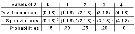
Variance = \( \sigma^2_x = (0 - 1.8)^2(0.15) + (1-1.8)^2(0.3) + (2-1.8)^2(0.25) + (3-1.8)^2(0.2) + (4-1.8)^2(0.1) = 1.46 \)
Standard deviation = \( \mu_x = \sqrt{1.46} = 1.21 \)
Q. How do we interpret the standard deviation of X?
Xavier's production line produces an average of 1.80 defective parts per hour. The number of defective parts varies from hour to hour; typically (or, on average), it is about 1.21 away from 1.80.
Here is the formal definition: standard deviation of a discrete random variable (definition) For any discrete random variable X with a probability distribution of
-
the variance of X is defined to be \( \sigma^2_x = (x_1 - \mu_x)^2p_1 + (x_2 - \mu_x)^2p_2 + ... + (x_n - \mu_x)^2p_n\)
\( = \sum_{i=1}^n (x_i - \mu_x)^2p_i \) and the standard deviation is \( \sigma_x = \sqrt{\sigma^2_x} \)
Solve the following
- Explanation :
Indeed, the probability distribution of the random variable W is centered at the mean of 3, and the typical distance between the values that W can have (1,5) and the mean 3 is 2.
- Explanation :
Indeed, the probability distribution of the random variable X is centered at the mean of 4, and the typical distance between the values that X can have and the mean is 1.
- Explanation :
Indeed, the probability distribution of the random variable Y is centered at the mean of 3, and the typical distance between the values that Y can have and the mean is 1.
- Explanation :
Indeed, the probability distribution of the random variable Z is centered at the mean of 4, and the typical distance between the values that Z can have and the mean is 2.
SubmitSubmit Your Answer
Standard Deviation of a Random Variable: Examples
Example: Xavier's and Yves' Production Lines : Recall the probability distribution of the random variable X, representing the number of defective parts per hour produced by Xavier's production line, and the probability distribution of the random variable Y, representing the number of defective parts per hour produced by Yves' production line:
Look carefully at both probability distributions. Both X and Y take the same possible values (0, 1, 2, 3, 4). However, they are very different in the way the probability is distributed among these values. We saw before that this makes a difference in means: \( \mu_X = 1.8, \mu_Y = 2.7 \) We now want to get a sense about how the different probability distributions impact their standard deviations. Recall that the standard deviation of a random variable can be interpreted as a typical (or the long-run average) distance between the value of X and its mean.
So, 75% of the time, Y will assume a value (3) that is very close to its mean (2.7), while X will assume a value (2) that is close to its mean (1.8) much less often—only 25% of the time. The long-run average, then, of the distance between the values of Y and their mean will be much smaller than the long-run average of the distance between the values of X and their mean.
Therefore, \( \sigma_Y < \sigma_X = 1.21 \) Actually, \( \sigma_Y = 0.85 \) , so we can draw the following conclusion:
Yves' production line produces an average of 2.70 defective parts per hour. The number of defective parts varies from hour to hour; typically (or, on average), it is about 0.85 away from 2.70.
Here are the histograms for the production lines:
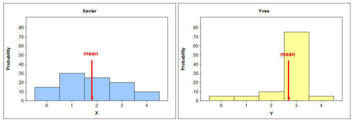
When we compare distributions, the distribution in which it is more likely to find values that are further from the mean will have a larger standard deviation. Likewise, the distribution in which it is less likely to find values that are further from the mean will have the smaller standard deviation.
- Explanation :
The probabilities of the values that are further from the mean are larger in Xavier's distribution than in Yves', making them more likely.
- Explanation :
When it is more likely (probable) to find values further from the mean, it is more likely that the standard deviation will be larger.
- Explanation :
Note that 75% of the time, Y will get the value 3, which is very close to its mean (2.7). On the other hand, only 25% of time will X get the value 2, which is very close to its mean (1.8).
The following graphs will be used to answer this question.
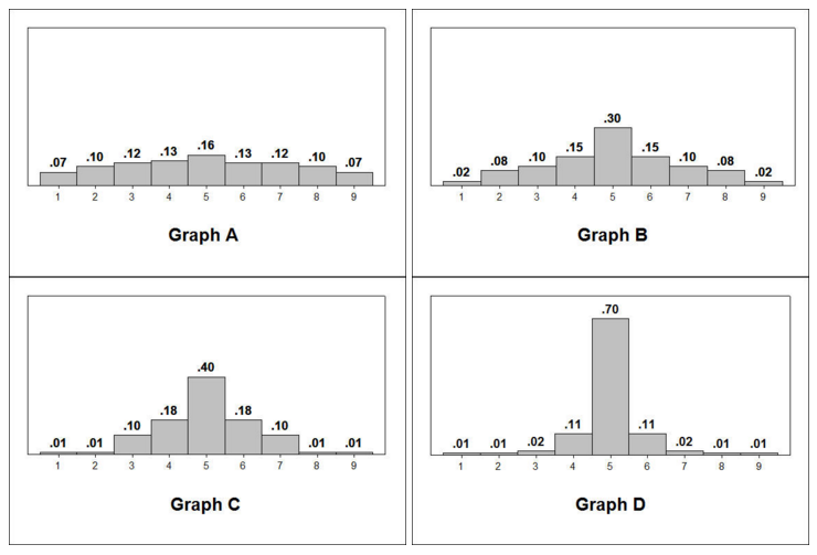
- Explanation :
This distribution has the largest spread relative to the mean, with higher relative frequencies that are further from the mean than the other distributions.
Example: Xavier's Production Line—Unusual or Not?
As we have stated before, using the mean and standard deviation gives us another way to assess which values of a random variable are unusual. Any values of a random variable that fall within 2 standard deviations of the mean would be considered ordinary (not unusual).
Would it be considered unusual to have 4 defective parts per hour?
We know that \( \mu_X = 1.8, \sigma_x = 1.21 \) .
Ordinary values are within 2 standard deviations of the mean. 1.8 - 2(1.21) = -0.62 and 1.8 + 2(1.21) = 4.22. This gives us an interval from -0.62 to 4.22. Since we cannot have a negative number of defective parts, the interval is essentially from 0 to 4.22. Because 4 is within this interval, it would be considered ordinary. Therefore, it is not unusual.
Would it be considered unusual to have no defective parts? Zero is within 2 standard deviations of the mean, so it would not be considered unusual to have no defective parts.
From the probability distribution for changing majors. We have made the following calculations for the mean and standard deviation. \( \mu_X = 1.23 and \sigma_X = 1.08\)
John's parents are concerned because John is changing majors for the second time. John claims this is not unusual. Using the mean and standard deviation given above, is John's behavior unusual?
Since the mean is 1.23 and the standard deviation is 1.08, two changes is less than 1 standard deviation above the mean. 1.23 + 1.08 = 2.31 So, John's behavior is not unusual at all. In fact, it is quite ordinary.
"Risk" in investments provides a useful application for the concept of variability. If there is no variability at all in possible outcomes, then the outcome is something we can count on, with no risk involved. At the other extreme, if there is a large amount of variability with possibilities for either tremendous loss or gain, then the associated risk is quite high.
If a variable's possible values just differ somewhat, with some only marginally favorable and others unfavorable, then the underlying random experiment entails just a moderate amount of risk. The following example demonstrates how differing values of standard deviation reflect the amount of risk in a situation.
Example: Comparing Investments
Consider three possible investments, with returns denoted as X, Y, and Z, respectively, and probability distributions outlined in the tables below.
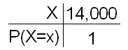
Investment X is what we'd call a "sure thing," with a guaranteed return of $14,000: there is no risk involved at all.
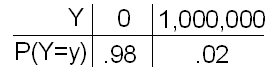
Investment Y is extremely risky, with a high probability (.98) of no gain at all, contrasted by a slight probability (.02) of "making a killing" with a return of a million dollars.
Investment Z is somewhere in between: there is an equal chance of either a return that's on the low side or a return that's on the high side.
If you only consider the mean return on each investment, would you prefer X, Y, or Z? The means for X, Y, and Z are calculated as follows:
\( \mu_X = 14000*1 = 14000 \)
\( \mu_Y = 0(0.98) + 1000000(0.02) = 20000 \)
\( \mu_Z = 10000(0.5) + 20000(0.5) = 15000 \)
Clearly, the mean return for Y is highest, and so investment in Y would seem to be preferable.
Now consider the standard deviations, and consider which investment you'd prefer — X, Y, or Z.
The standard deviations are:
\( \sigma^2_x = (14000 - 14000)^2(1) = 0 \)
\( \sigma_x = 0 \)
\( \sigma^2_y = (0 - 20000)^2(0.98) + (1000000 - 20000)^2(0.02) = 1.96 * 10^10\)
\( \sigma_Y = 140000 \)
\( \sigma^2_Z = (10000 - 15000)^2(0.5) + (20000 - 15000)^2(0.5) = 25000000\)
\( \sigma_z = 5000 \)
Granted, the mean returns suggest that investment X is least profitable and investment Y is most profitable. On the other hand, the standard deviations are telling us that the return for X is a sure thing; for Y, the remote chance of making a huge profit is offset by a high risk of losing the investment entirely; for Z, there is a modest amount of risk involved.
If you can't afford to lose any money, then investment X would be the way to go. If you have enough assets to take a big chance, then investment Y would be worthwhile.
In particular, if a large company routinely makes many such investments, then in the long run there will occasionally be such enormous gains that the company is willing to absorb many smaller losses. Investment Z represents the middle ground, somewhere between the other two.
Rules for Means and Variances of Random Variables: Add, Subtract, Multiply by a Constant - Example: Xavier's Production Line
Assume that operating Xavier's production line costs $50 per hour, and that the repair cost of one defective part is $5. If X is the number of defective parts produced per hour, then the hourly cost would be 50 + 5X. Note that since X is a random variable, so is the cost, 50 + 5X, and we might be interested in the mean and standard deviation of the hourly cost of operation for Xavier's production line.
If we know the mean and standard deviation for the number of defective parts (X), is there an easy way to find the mean and standard deviation for the hourly cost (50 + 5X)?
In General Sometimes a new random variable of interest arises when we take an existing random variable and multiply by a constant and/or add a constant to its values. In the example above, we both multiplied X by 5 and added 50. We will return to the above example after exploring how such changes affect the center (mean) and spread (standard deviation) of random variables in general.
Consider the random variable X with a probability distribution as shown in the histogram below:
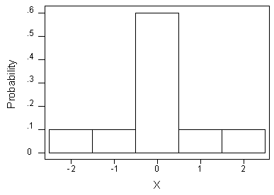
It can easily be shown that X has a mean of 0, and a standard deviation of 1.
Adding a Constant to X What would the mean and standard deviation be if we shifted the entire histogram over 6 units to the right—in other words, what are the mean and standard deviation of X + 6?
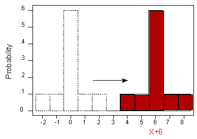
We observe that shifting the distribution over to the right 6 units also shifts the center over 6 units: in other words, the mean of (X + 6) should equal the (mean of X) + 6. However, the spread of the distribution is unchanged: in other words, the standard deviation of (X + 6) should equal the standard deviation of X.
Again consider the random variable X with the probability distribution shown in the histogram below:
-
Subtracting a Constant from X What would the mean and standard deviation be if we shifted the entire histogram over 7 units to the left—in other words, what are the mean and standard deviation of X - 7?
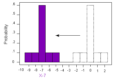
The mean also shifts to the left by 7, from 0 to -7. The standard deviation remains unchanged at 1.
Multiplying X by a Constant That Is > 1 What would the mean and standard deviation be if we stretched the entire histogram by 4 units—in other words, what are the mean and standard deviation of 4X?
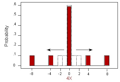
Multiplying X by 4 results in a mean that is 4 times the original mean. In this case, the mean transforms from 0 to 4(0) = 0. Multiplying X by 4 is tantamount to stretching the distribution by 4 units, and so the standard deviation will be 4 times the original standard deviation. In other words, the mean of 4X is 4 times the mean of X; the standard deviation of 4X is 4 times the standard deviation of X. The variance, or squared standard deviation, would be 4 squared times the original variance; the variance of 4X is 16 times the variance of X.
Multiplying X by a Constant That Is < 1 Finally, what would the mean and standard deviation be if we shrunk the entire histogram by a fourth—in other words, what are the mean and standard deviation of (1/4) X?
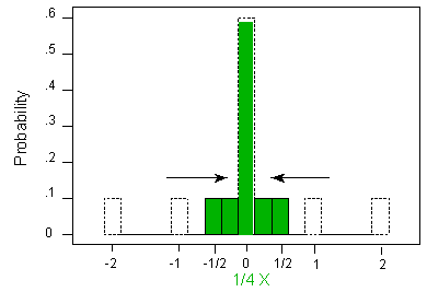
Dividing X by 4 results in a mean that is 1/4 the original mean. In this case, the mean transforms from 0 to (1/4)(0) = 0. Dividing X by 4 is tantamount to shrinking the distribution by 4 units, and so the standard deviation will be 1/4 of the original standard deviation. In other words, the mean of (1/4)X is 1/4 times the mean of X; the standard deviation of (1/4)X is 1/4 times the standard deviation of X.
The variance, or squared standard deviation, would be 1/4 squared times the original variance; the variance of (1/4)X is 1/16 times the variance of X.
Rules for Means and Variances of Random Variables: Linear Transformation
The four observations we made on the previous page help illustrate a general rule for how random variables transform if we add, subtract and/or multiply by a constant.
Rules for a + bX (Linear Transformation of One Random Variable) If X is a random variable with the mean \( \mu_X \) and a variance of \( \sigma^2_x \), then the new random variable a + bX has a mean and variance (respectively) of: \( \mu_{a + bX} = a + b\mu_X \) \( \sigma^2_{a + bX} = b^2\sigma^2_x\)
Comment : If we take a random variable's distribution and shift it over "a" units, and stretch or shrink its spread by "b" (stretch if b is greater than 1, shrink if b is less than 1), then the mean is shifted and the distribution is stretched or shrunk accordingly.
For instance, if we multiply a random variable by 6 and add 3, then the mean is also transformed. The mean is also multiplied by 6 and 3 is added.
Shifting by "a," however, has no effect on the variance (or standard deviation) of a random variable, because the spread would not be changed. On the other hand, stretching or shrinking the distribution of a random variable entails stretching or shrinking its spread accordingly.
Doubling a random variable's values produces a new random variable whose variance is four times the original variance, but the standard deviation is just double the original standard deviation, as we might expect.
Example: Shifting and Stretching
Recall that X is the number of defective parts per hour in Xavier's production line, and in the previous section we calculated that:
\( \mu_x = 1.8 \) and that \( \sigma_x = 1.21 \).
We are interested in a new random variable, "50 + 5X," which represents the hourly cost of operation for Xavier's production line. Note that 50 + 5X is of the form "a + bX" (where a = 50 and b = 5), so in order to find the mean and standard deviation of this new random variable, we can use the rules above:
\( \mu_{50+5x} = 50 + 5\mu_x = 50 + 5(1.8) = 59 \)
\( \sigma^2_{50+5x} = 5^2\sigma^2_x = 25(1.46) = 36.5 \)
and therefore: \( \sigma_{50+5x} = \sqrt{36.5} = 6.04 \)
So, we can conclude that the hourly costs for Xavier's production line average $59, and typically the cost is about $6 away from that average.
- Explanation :
There is a $3 charge per car (regardless of the number of people in the car), plus $.50 for each person in the car.
- Explanation :
Indeed, μ3+50X = 3 + 0.50 * μX = 3 + 0.50 * 2.7 = 4.35, and σ23+0.50X = 0.502 * σ2X = 0.25 * 1.2 = 0.30. Therefore, the standard deviation is sqrt(0.30).
Rules for Means and Variances of Random Variables: Sum of Two Variables
Besides taking a linear transformation of a random variable, another way to form a new random variable is to combine two or more existing random variables in some way, such as finding the sum of two random variables. Again, we'll start with a motivating example.
Example: Xavier's and Yves' Production Lines Recall previous examples for the number X of defective parts coming out of Xavier's production line, and Y from Yves' line. Consider the total number of defective parts coming out of both production lines together. This is the new random variable X + Y. Since we know the means and standard deviations of X and of Y, is there a simple, quick way to figure out the mean and standard deviation of X + Y?
In general, the mean of the sum of random variables is the sum of the means. As long as the random variables are independent, the variance of the sum equals the sum of the variances. The formal rules are as follows:
Rules for X + Y (Sum of Two Random Variables) Let X and Y be random variables with means \( \mu_x \) and \( \mu_y \) and with variances \( \sigma^2_x \) and \( \sigma^2_y \). Then the new random variable X + Y has a mean of
\( \mu_{x+y} = \mu_x + \mu_y \)
and as long as the random variables are independent, the variance of X + Y is:
\( \sigma^2_{x+y} = \sigma^2_x + \sigma^2_y \)
What these two rules tell us is that if we take two random variables and add them, then the new mean is the sum of the original two means, and the new variance—not standard deviation—is the sum of the original two variances, as long as those variables are independent.
Comment We've talked a lot about independent and dependent events, but not about what it means for two random variables to be independent or dependent. Basically, the same reasoning extends from events to random variables. Two random variables will be independent if knowing that one random variable takes any of its possible values has no effect on the probability that the other random variable takes a certain value.
While in the case of events we formalized the definition of independence using conditional probability, doing the same for random variables is beyond the scope of this course. Therefore, whenever we want to use the rule:
\( \sigma^2_{x+y} = \sigma^2_x + \sigma^2_y \) , we will assume that X and Y are independent, or it will be clear from the context of the problem.
Example: Combined Mean and Standard Deviation We want to find the mean and standard deviation of X + Y, the total number of defective products coming out of both production lines in an hour. In the previous section, we found that:
\( \mu_x = 1.8, \sigma_x = 1.21, \mu_y = 2.7 and \sigma_y = 0.85 \)
Using the rules for X + Y, we find that:
\( \mu_{x+y} = \mu_x + \mu_y = 1.8 + 2.7 = 4.5 \)
\( \sigma^2_{x+y} = \sigma^2_x + \sigma^2_y = 1.21^2 + 0.85^2 = 2.19 \)
\( \sigma_{x+y} = \sqrt{2.19} = 1.48 \)
We can conclude, then, that the total number of defective parts coming out of both production lines in an hour is on average 4.5, and typically the combined number of defective products is about 1.48 away from that average.
Comment It is important to remember that while variances are additive, standard deviations are not: \( \sigma_x + \sigma_y = 1.21 + 0.85 = 2.06 \neq \sigma{x+y} = 1.48 \)
- Explanation :
Indeed, since T = X + Y, μT = μX + μY = 25 + 35 = 60.
- Explanation :
Indeed, since X and Y are independent: σ2T = σ2X+Y = σ2X + σ2Y = 25 + 64 = 89. Therefore σT is the square root of 89.
- Explanation :
Let T be the total cost of manufacturing monitors for a day. T is composed of two parts: the fixed cost of $500 (regardless of the number of monitors) and $15 for every monitor made. The total cost can be written as T = 500 + 15X. To find the mean of T you use the rule of means: μ(a+bX) = a + b μx = 500 + 15(120) = $2300.
- Explanation :
Since Z = X + Y, μZ = μx + μy = 23 + 18 = 41.