When we explore the relationship between two variables, there is often a temptation to conclude from the observed relationship that changes in the explanatory variable cause changes in the response variable.

In other words, you might be tempted to interpret the observed association as causation. The purpose of this part of the course is to convince you that this kind of interpretation is often wrong! The motto of this section is one of the most fundamental principles of this course: Association does not imply causation!

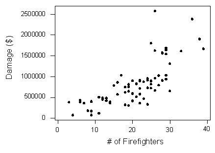
The scatterplot below illustrates how the number of firefighters sent to fires (X) is related to the amount of damage caused by fires (Y) in a certain city.

The scatterplot clearly displays a fairly strong (slightly curved) positive relationship between the two variables. Would it, then, be reasonable to conclude that sending more firefighters to a fire causes more damage, or that the city should send fewer firefighters to a fire, in order to decrease the amount of damage done by the fire? Of course not!

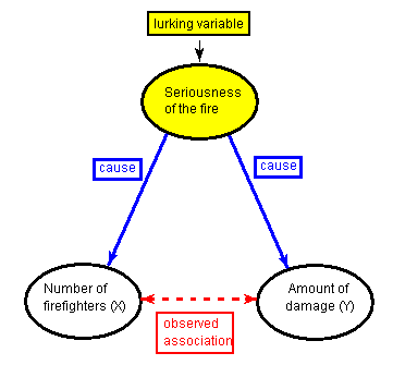
There is a third variable in the background—the seriousness of the fire—that is responsible for the observed relationship. More serious fires require more firefighters, and also cause more damage.

Here, the seriousness of the fire is a lurking variable. A lurking variable is a variable that is not among the explanatory or response variables in a study, but could substantially affect your interpretation of the relationship among those variables.

In particular, as in our example, the lurking variable might have an effect on both the explanatory and the response variables. This common effect creates the observed association between the explanatory and response variables, even though there is no causal link between them.

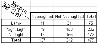
When we practiced exploring the relationship between two categorical variables, we looked at a study in which the type of light in young children's rooms when they sleep was examined, along with their later nearsightedness, or myopia. Here is the two-way table that summarizes the collected data:

The conditional percentages allow us to compare the distribution of later nearsightedness among children who were exposed to each of the three nighttime light levels:

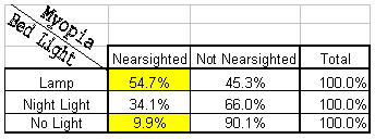
The striking finding was that children who slept with lamps on were more than 5 times more likely to be nearsighted later in life (54.7% vs. 9.9%). Based upon this data alone, parents might discontinue using night-lights and lamps with young children.

Do the data provide evidence that early light exposure causes myopia?

Association does not imply causation. We cannot conclude that light exposure in early childhood somehow causes myopia in older children. The data is suggestive of a relationship, but we can't rule out the possibility that a lurking variable is associated with parents' use of light with their young children and the children's later myopia.

What is a likely lurking variable in this case that could explain this observed relationship? (Hint: this lurking variable affects both the type of light with which a child sleeps and the child's later nearsightedness.)

A lurking variable that can very likely explain the observed relationship in this case is the nearsightedness of the child's parents (one or both). If the parents are nearsighted, then their child is more likely to be nearsighted due to genetic factors. Also, nearsighted parents are more likely to leave more light near their sleeping children to make it easier to care for them at night. Click here to see a visual explanation of this.

As you recall, a lurking variable, by definition, is a variable that was not included in the study, but could have a substantial effect on our understanding of the relationship between the two studied variables.

Example: Hospital Death Rates

Background : A government study collected data on the death rates in nearly 6,000 hospitals in the United States. These results were then challenged by researchers, who said that the federal analyses failed to take into account the variation among hospitals in the severity of patients' illnesses when they were hospitalized.

As a result, said the researchers, some hospitals were treated unfairly in the findings, which named hospitals with higher-than-expected death rates. What the researchers meant is that when the federal government explored the relationship between the two variables—hospital and death rate—it also should have included in the study (or taken into account) the lurking variable—severity of illness.

Consider the following two-way table, which summarizes the data about the status of patients who were admitted to two hospitals in a certain city (Hospital A and Hospital B). Note that since the purpose of the study is to examine whether there is a "hospital effect" on patients' status, "Hospital is the explanatory variable, and "Patient's Status" is the response variable.

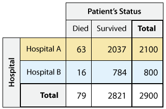
When we supplement the two-way table with the conditional percents within each hospital:

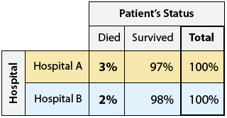
we find that Hospital A has a higher death rate (3%) than Hospital B (2%). Should we jump to the conclusion that a sick patient admitted to Hospital A is 50% more likely to die than if he/she were admitted to Hospital B? Not so fast ...

Maybe Hospital A gets most of the severe cases, and that explains why it has a higher death rate. In order to explore this, we need to include (or account for) the lurking variable "severity of illness" in our analysis. To do this, we go back to the two-way table and split it up to look separately at patents who are severely ill, and patients who are not.

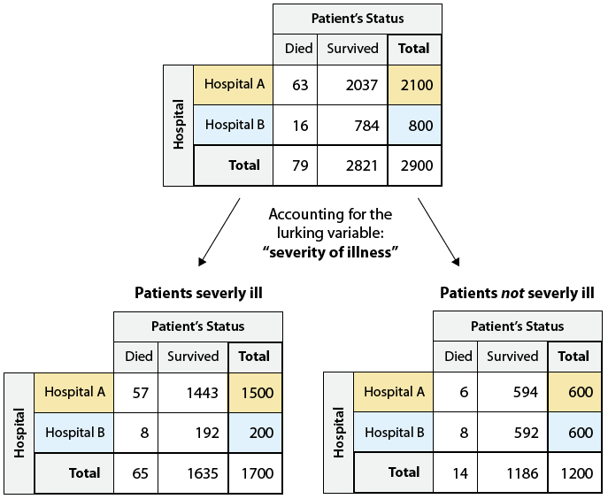
As we can see, Hospital A did admit many more severely ill patients than Hospital B (1,500 vs. 200). In fact, from the way the totals were split, we see that in Hospital A, severely ill patients were a much higher proportion of the patients—1,500 out of a total of 2,100 patients. In contrast, only 200 out of 800 patients at Hospital B were severely ill. To better see the effect of including the lurking variable, we need to supplement each of the two new two-way tables with its conditional percentages:

Note that despite our earlier finding that overall Hospital A has a higher death rate (3% vs. 2%), when we take into account the lurking variable, we find that actually it is Hospital B that has the higher death rate both among the severely ill patients (4% vs. 3.8%) and among the not severely ill patients (1.3% vs. 1%). Thus, we see that adding a lurking variable can change the direction of an association.

Whenever including a lurking variable causes us to rethink the direction of an association, this is called Simpson's paradox.

The following scatterplot displays the relationship between the percentage of students taking the SAT and the median SAT Math scores in each of the fifty states.

Note that the explanatory variable is the percent taking the SAT in each of the 50 states and the response variable is the SAT Math median score in each of the states.

Each data point on the scatterplot represents one of the states.

For example, in Illinois in the year these data were collected, 16 percent of the students took the SAT and the median score on the math part was 528. Notice that there is a negative relationship between the percentage of students who take the SAT in a state and the median SAT Math score in that state.

What could the explanation behind this negative trend be? Why might having more people taking the test be associated with lower scores?

Note that another visible feature of the data is the presence of a gap in the middle of the scatterplot which creates two distinct clusters in the data.

This suggests that maybe there is a lurking variable that separates the states into these two clusters and that including this lurking variable in the study, as we did by creating this labeled scatterplot, will help us understand the negative trend.

It turns out that indeed the two clusters represent two groups. The blue group on the right represents the states where the SAT is the test of choice for students and colleges.

And the red group on the left representing the states where the ACT college entrance examination is commonly used.

It makes sense, then, that in the ACT states on the left a smaller percentage of the students take the SAT.

Moreover those students who do take the SAT in those states are probably students who are applying to more prestigious national colleges and therefore represent a more selective group of students.

This is the reason why we see high SAT Math scores in this group. On the other hand in the SAT states on the right, larger percentages of students take the SAT.

These students represent a much broader cross-section of the population and therefore we see lower SAT Math scores.

To summarize, in this case including the lurking variable ACT State vs SAT State helped us better understand the observed negative relationship in our data.

A lurking variable is a variable that was not included in your analysis, but that could substantially change your interpretation of the data if it were included.

Because of the possibility of lurking variables, we adhere to the principle that association does not imply causation.

Including a lurking variable in our exploration may: help us to gain a deeper understanding of the relationship between variables, or lead us to rethink the direction of an association.

Whenever including a lurking variable causes us to rethink the direction of an association, this is an instance of Simpson's paradox.