Setting Up Your Programming Assignment Environment
Introductory Video
The Machine Learning course includes several programming assignments which you’ll need to finish to complete the course. The assignments require the Octave scientific computing language.
Octave is a free, open-source application available for many platforms. It has a text interface and an experimental graphical one. Octave is distributed under the GNU Public License, which means that it is always free to download and distribute.
Use Download to install Octave for windows. "Warning: Do not install Octave 4.0.0";
Installing Octave on GNU/Linux : On Ubuntu, you can use: sudo apt-get update && sudo apt-get install octave. On Fedora, you can use: sudo yum install octave-forge
Introduction
In this exercise, you will implement Support Vector Machines.
Files included in this exercise can be downloaded here ⇒ : Download
In this exercise, you will be using support vector machines (SVMs) to build a spam classifier. Before starting on the programming exercise, we strongly recommend watching the video lectures and completing the review questions for the associated topics.
To get started with the exercise, you will need to download the starter code and unzip its contents to the directory where you wish to complete the exercise. If needed, use the cd command in Octave/MATLAB to change to this directory before starting this exercise.
You can also find instructions for installing Octave/MATLAB in the “Environment Setup Instructions” above.
Files included in this exercise
ex6.m - Octave/MATLAB script for the first half of the exercise
ex6data1.mat - Example Dataset 1
ex6data2.mat - Example Dataset 2
ex6data3.mat - Example Dataset 3
svmTrain.m - SVM training function
svmPredict.m - SVM prediction function
plotData.m - Plot 2D data
visualizeBoundaryLinear.m - Plot linear boundary
visualizeBoundary.m - Plot non-linear boundary
linearKernel.m - Linear kernel for SVM
[*] gaussianKernel.m - Gaussian kernel for SVM
[*] dataset3Params.m - Parameters to use for Dataset 3
ex6 spam.m - Octave/MATLAB script for the second half of the exercise
spamTrain.mat - Spam training set
spamTest.mat - Spam test set
emailSample1.txt - Sample email 1
emailSample2.txt - Sample email 2
spamSample1.txt - Sample spam 1
spamSample2.txt - Sample spam 2
vocab.txt - Vocabulary list
getVocabList.m - Load vocabulary list
porterStemmer.m - Stemming function
readFile.m - Reads a file into a character string
submit.m - Submission script that sends your solutions to our servers
[*] processEmail.m - Email preprocessing
[*] emailFeatures.m - Feature extraction from emails
* indicates files you will need to complete Throughout the exercise, you will be using the script ex6.m. These scripts set up the dataset for the problems and make calls to functions that you will write. You are only required to modify functions in other files, by following the instructions in this assignment.
Support Vector Machines - Example Dataset 1
In the first half of this exercise, you will be using support vector machines (SVMs) with various example 2D datasets. Experimenting with these datasets will help you gain an intuition of how SVMs work and how to use a Gaussian kernel with SVMs.
In the next half of the exercise, you will be using support vector machines to build a spam classifier. The provided script, ex6.m, will help you step through the first half of the exercise
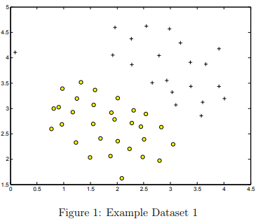
We will begin by with a 2D example dataset which can be separated by a linear boundary.
The script ex6.m will plot the training data (Figure 1). In this dataset, the positions of the positive examples (indicated with +) and the negative examples (indicated with o) suggest a natural separation indicated by the gap. However, notice that there is an outlier positive example + on the far left at about (0.1, 4.1).
As part of this exercise, you will also see how this outlier affects the SVM decision boundary.
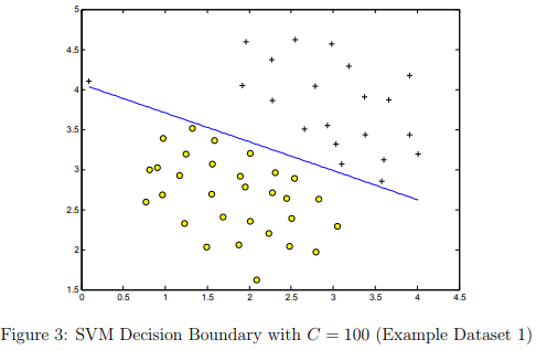
In this part of the exercise, you will try using different values of the C parameter with SVMs. Informally, the C parameter is a positive value that controls the penalty for misclassified training examples.
A large C parameter tells the SVM to try to classify all the examples correctly. C plays a role similar to 1/λ, where λ is the regularization parameter that we were using previously for logistic regression.
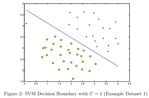
The next part in ex6.m will run the SVM training (with C = 1) using SVM software that we have included with the starter code, svmTrain.m.
When C = 1, you should find that the SVM puts the decision boundary in the gap between the two datasets and misclassifies the data point on the far left (Figure 2).
Implementation Note: Most SVM software packages (including svmTrain.m) automatically add the extra feature x0 = 1 for you and automatically take care of learning the intercept term θ0.
So when passing your training data to the SVM software, there is no need to add this extra feature x0 = 1 yourself.
In particular, in Octave/MATLAB your code should be working with training examples x ∈ Rn (rather than x ∈ Rn+1; for example, in the first example dataset x ∈ R2
Your task is to try different values of C on this dataset. Specifically, you should change the value of C in the script to C = 100 and run the SVM training again. When C = 100, you should find that the SVM now classifies every single example correctly, but has a decision boundary that does not appear to be a natural fit for the data (Figure 3).
SVM with Gaussian Kernels
In this part of the exercise, you will be using SVMs to do non-linear classification. In particular, you will be using SVMs with Gaussian kernels on datasets that are not linearly separable.
Gaussian Kernel To find non-linear decision boundaries with the SVM, we need to first implement a Gaussian kernel. You can think of the Gaussian kernel as a similarity function that measures the “distance” between a pair of examples, (x(i), x(j)).
The Gaussian kernel is also parameterized by a bandwidth parameter, σ, which determines how fast the similarity metric decreases (to 0) as the examples are further apart.
You should now complete the code in gaussianKernel.m to compute the Gaussian kernel between two examples, (x(i), x(j)). The Gaussian kernel function is defined as:
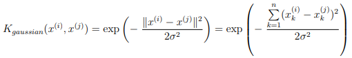
Once you’ve completed the function gaussianKernel.m, the script ex6.m will test your kernel function on two provided examples and you should expect to see a value of 0.324652.
SVM with Gaussian Kernels- Tutorials
gaussianKernel(): The method is similar to that used for sigmoid.m in ex2. The numerator is the sum of the squares of the difference of two vectors. That's just like computing the linear regression cost function. Use exp() and scale by the value given in the formula
SVM with Gaussian Kernels - Testcases
gaussianKernel([1 2 3], [2 4 6], 3)

% result
ans =  0.45943

% Verify that the same point returns 1
>> gaussianKernel([1 1], [1 1], 1)

ans =

     1

% Verify that disimilar points return 0 (or close to it)
>> gaussianKernel([1 1], [100 100], 1)

ans =

     0
SVM with Gaussian Kernels - Example Dataset 2
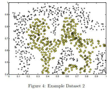
The next part in ex6.m will load and plot dataset 2 (Figure 4).From the figure, you can obserse that there is no linear decision boundary that separates the positive and negative examples for this dataset.
However, by using the Gaussian kernel with the SVM, you will be able to learn a non-linear decision boundary that can perform reasonably well for the dataset.
If you have correctly implemented the Gaussian kernel function, ex6.m will proceed to train the SVM with the Gaussian kernel on this dataset.
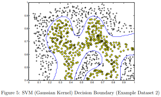
Figure 5 shows the decision boundary found by the SVM with a Gaussian kernel. The decision boundary is able to separate most of the positive and negative examples correctly and follows the contours of the dataset well.
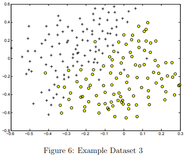
Example Dataset 3
In this part of the exercise, you will gain more practical skills on how to use a SVM with a Gaussian kernel. The next part of ex6.m will load and display a third dataset (Figure 6). You will be using the SVM with the Gaussian kernel with this dataset.
In the provided dataset, ex6data3.mat, you are given the variables X, y, Xval, yval. The provided code in ex6.m trains the SVM classifier using the training set (X, y) using parameters loaded from dataset3Params.m. Your task is to use the cross validation set Xval, yval to determine the best C and σ parameter to use.
You should write any additional code necessary to help you search over the parameters C and σ. For both C and σ, we suggest trying values in multiplicative steps (e.g., 0.01, 0.03, 0.1, 0.3, 1, 3, 10, 30).
Note that you should try all possible pairs of values for C and σ (e.g., C = 0.3 and σ = 0.1).
For example, if you try each of the 8 values listed above for C and for σ2 , you would end up training and evaluating (on the cross validation set) a total of 82 = 64 different models.
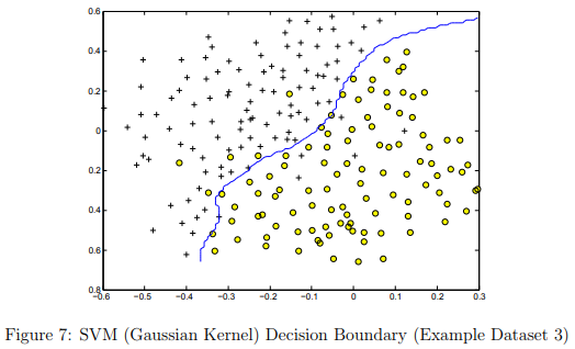
After you have determined the best C and σ parameters to use, you should modify the code in dataset3Params.m, filling in the best parameters you found.
For our best parameters, the SVM returned a decision boundary shown in Figure 7.
Implementation Tip: When implementing cross validation to select the best C and σ parameter to use, you need to evaluate the error on the cross validation set. Recall that for classification, the error is defined as the fraction of the cross validation examples that were classified incorrectly. In Octave/MATLAB, you can compute this error using mean(double(predictions ~= yval)), where predictions is a vector containing all the predictions from the SVM, and yval are the true labels from the cross validation set. You can use the svmPredict function to generate the predictions for the cross validation set
Example Dataset 3 - dataset3Params(): Tutorial
One method is to use two nested for-loops - each one iterating over the range of C or sigma values given in the ex6.pdf file.
Inside the inner loop: Train the model using svmTrain with X, y, a value for C, and the gaussian kernel using a value for sigma. See ex6.m at line 108 for an example of the correct syntax to use in calling svmTrain() and the gaussian kernel.
Note: Use temporary variables for C and sigma when you call svmTrain(). Only use 'C' and 'sigma' for the final values you are going to return from the function. Compute the predictions for the validation set using svmPredict() with model and Xval.
Compute the error between your predictions and yval. When you find a new minimum error, save the C and sigma values that were used. Or, for each error computation, you can save the C, sigma, and error values as rows of a matrix.
When all 64 computations are completed, use min() to find the row with the minimum error, then use that row index to retrieve the C and sigma values that produced the minimum error.
Example Dataset 3 - dataset3Params(): Testcases
x1plot = linspace(-2, 2, 10)';
x2plot = linspace(-2, 2, 10)';
[X1, X2] = meshgrid(x1plot, x2plot);
X = [X1(:) X2(:)];
Xval = X + 0.3;
y = double(sum(exp(X),2) > 3);
yval = double(sum(exp(Xval),2) > 3);
[C sigma] = dataset3Params(X, y, Xval, yval)

% best C and sigma:
C = 0.1
sigma = 1.0

% table of results for selected C and sigma
   Errors      C        sigma
   0.06000   0.10000   0.10000
   0.04000   0.10000   0.30000
   0.00000   0.10000   1.00000
   0.06000   0.30000   0.10000
   0.04000   0.30000   0.30000
   0.04000   0.30000   1.00000
   0.06000   1.00000   0.10000
   0.04000   1.00000   0.30000
   0.02000   1.00000   1.00000
Spam Classification - Preprocessing Emails
Many email services today provide spam filters that are able to classify emails into spam and non-spam email with high accuracy. In this part of the exercise, you will use SVMs to build your own spam filter.
You will be training a classifier to classify whether a given email, x, is spam (y = 1) or non-spam (y = 0). In particular, you need to convert each email into a feature vector x ∈ Rn .
The following parts of the exercise will walk you through how such a feature vector can be constructed from an email.
Throughout the rest of this exercise, you will be using the the script ex6 spam.m. The dataset included for this exercise is based on a a subset of the SpamAssassin Public Corpus. (http://spamassassin.apache.org/old/publiccorpus/ )
For the purpose of this exercise, you will only be using the body of the email (excluding the email headers).
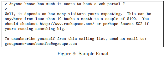
Before starting on a machine learning task, it is usually insightful to take a look at examples from the dataset. Figure 8 shows a sample email that contains a URL, an email address (at the end), numbers, and dollar amounts.
While many emails would contain similar types of entities (e.g., numbers, other URLs, or other email addresses), the specific entities (e.g., the specific URL or specific dollar amount) will be different in almost every email.
Therefore, one method often employed in processing emails is to “normalize” these values, so that all URLs are treated the same, all numbers are treated the same, etc. For example, we could replace each URL in the email with the unique string “httpaddr” to indicate that a URL was present.
This has the effect of letting the spam classifier make a classification decision based on whether any URL was present, rather than whether a specific URL was present.
This typically improves the performance of a spam classifier, since spammers often randomize the URLs, and thus the odds of seeing any particular URL again in a new piece of spam is very small.
In processEmail.m, we have implemented the following email preprocessing and normalization steps:
Lower-casing: The entire email is converted into lower case, so that captialization is ignored (e.g., IndIcaTE is treated the same as Indicate).
Stripping HTML: All HTML tags are removed from the emails. Many emails often come with HTML formatting; we remove all the HTML tags, so that only the content remains.
Normalizing URLs: All URLs are replaced with the text “httpaddr”.
Normalizing Email Addresses: All email addresses are replaced with the text “emailaddr”.
Normalizing Numbers: All numbers are replaced with the text “number”.
Normalizing Dollars: All dollar signs ($) are replaced with the text “dollar”.
Word Stemming: Words are reduced to their stemmed form. For example, “discount”, “discounts”, “discounted” and “discounting” are all replaced with “discount”. Sometimes, the Stemmer actually strips off additional characters from the end, so “include”, “includes”, “included”, and “including” are all replaced with “includ”.
Removal of non-words: Non-words and punctuation have been removed. All white spaces (tabs, newlines, spaces) have all been trimmed to a single space character.
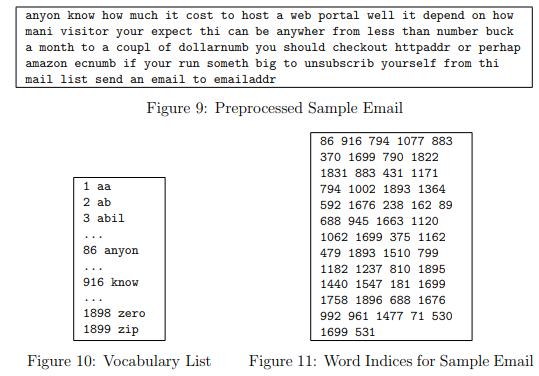
The result of these preprocessing steps is shown in Figure 9. While preprocessing has left word fragments and non-words, this form turns out to be much easier to work with for performing feature extraction.
Vocabulary List
After preprocessing the emails, we have a list of words (e.g., Figure 9) for each email. The next step is to choose which words we would like to use in our classifier and which we would want to leave out.
For this exercise, we have chosen only the most frequently occuring words as our set of words considered (the vocabulary list). Since words that occur rarely in the training set are only in a few emails, they might cause the model to overfit our training set.
The complete vocabulary list is in the file vocab.txt and also shown in Figure 10. Our vocabulary list was selected by choosing all words which occur at least a 100 times in the spam corpus, resulting in a list of 1899 words.
In practice, a vocabulary list with about 10,000 to 50,000 words is often used.
Given the vocabulary list, we can now map each word in the preprocessed emails (e.g., Figure 9) into a list of word indices that contains the index of the word in the vocabulary list.
Figure 11 shows the mapping for the sample email. Specifically, in the sample email, the word “anyone” was first normalized to “anyon” and then mapped onto the index 86 in the vocabulary list.
Your task now is to complete the code in processEmail.m to perform this mapping. In the code, you are given a string str which is a single word from the processed email.
You should look up the word in the vocabulary list vocabList and find if the word exists in the vocabulary list. If the word exists, you should add the index of the word into the word indices variable.
If the word does not exist, and is therefore not in the vocabulary, you can skip the word.
Once you have implemented processEmail.m, the script ex6_spam.m will run your code on the email sample and you should see an output similar to Figures 9 & 11.
Octave/MATLAB Tip: In Octave/MATLAB, you can compare two strings with the strcmp function. For example, strcmp(str1, str2) will return 1 only when both strings are equal. In the provided starter code, vocabList is a “cell-array” containing the words in the vocabulary. In Octave/MATLAB, a cell-array is just like a normal array (i.e., a vector), except that its elements can also be strings (which they can’t in a normal Octave/MATLAB matrix/vector), and you index into them using curly braces instead of square brackets. Specifically, to get the word at index i, you can use vocabList{i}. You can also use length(vocabList) to get the number of words in the vocabulary.
Vocabulary List: processEmail(): Tutorial
Start by setting a breakpoint in the processEmail.m script template (use the code editor in the GUI), in the blank area below the "YOUR CODE HERE" comment block. Then run the ex6_spam script.
When program execution hits the breakpoint, it will activate the console in debug mode. There you can inspect the variables "str" and "vocabList" (type the variable name into the console and press
). Observe that str holds a single word, and that vocabList is a cell array of all known words. Resume execution with the 'return' command in the debugger.
For the code you need to add: Here is an example using the strcmp() function showing how to find the index of a word in a cell array of words:
small_list = {'alpha', 'bravo', 'charlie', 'delta', 'echo'}
match = strcmp('bravo', small_list)
find(match)
strcmp() returns a logical vector, with a 1 marking each location where a word occurs in the list. If there is no match, all of the logical values are 0's.
The find() function returns a list of the non-zero elements in "match". You can add these index values to the word_indices list by concatenation.
Note that if there is no match, find() returns a null vector, and this can be concatenated to the word list without any problems.
Note that your word_index list must be returned as a column vector. If you make it a row vector, the submit grader will still give you credit, but your emailFeatures() function will not work correctly.
Vocabulary List: processEmail(): Testcases
word_indices  = processEmail('abe above abil ab tip the cow')

==== Processed Email ====

ab abov abil ab tip the cow

=========================
word_indices =

      2
      6
      3
      2
   1695
   1666

Tip: If you get the wrong word index for the word 'the', verify that you are using strcmp(), not strfind().
Extracting Features from Emails
You will now implement the feature extraction that converts each email into a vector in Rn .
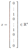
For this exercise, you will be using n = # words in vocabulary list. Specifically, the feature xi ∈ {0, 1} for an email corresponds to whether the i-th word in the dictionary occurs in the email.
That is, xi = 1 if the i-th word is in the email and xi = 0 if the i-th word is not present in the email.
Thus, for a typical email, this feature would look like:
You should now complete the code in emailFeatures.m to generate a feature vector for an email, given the word indices.
Once you have implemented emailFeatures.m, the next part of ex6 spam.m will run your code on the email sample. You should see that the feature vector had length 1899 and 45 non-zero entries.
Extracting Features from Emails emailFeatures: Tutorial
The emailFeatures() function is one of the simplest in the entire course:
You're given a list of word indexes. For each index in that list, you're asked to set the corresponding entries in an 'x' array to the value '1'.
A couple of different methods could be used: Loop through the list of word indexes, and use each index to set the corresponding value in the 'x' array to 1.
Take advantage of vectorized indexing, and do the same operation in one line of code without the loop.
Note that the 'x' feature list must be a column vector, and the word_indices list (which is provided by your processEmail() function) must be a column vector.
You can complete this function by adding only one line of code.Try this example in your console:
vec = zeros(10,1)     % included in the function template
indexes = [1 3 5]     % you're provided with a list of indexes
vec(indexes) = 1      % set the values to 1
Extracting Features from Emails emailFeatures: Testcases
% input
idx = [2 4 6 8 2 4 6 8]';
v = emailFeatures(idx);
v(1:10)
sum(v)

% results
>> v(1:10)
ans =
   0
   1
   0
   1
   0
   1
   0
   1
   0
   0

>> sum(v)
ans =  4
Training SVM for Spam Classification
After you have completed the feature extraction functions, the next step of ex6 spam.m will load a preprocessed training dataset that will be used to train a SVM classifier.
spamTrain.mat contains 4000 training examples of spam and non-spam email, while spamTest.mat contains 1000 test examples.
Each original email was processed using the processEmail and emailFeatures functions and converted into a vector x(i) ∈ R1899 .
After loading the dataset, ex6 spam.m will proceed to train a SVM to classify between spam (y = 1) and non-spam (y = 0) emails.
Once the training completes, you should see that the classifier gets a training accuracy of about 99.8% and a test accuracy of about 98.5%.
Top Predictors for Spam
-
To better understand how the spam classifier works, we can inspect the parameters to see which words the classifier thinks are the most predictive of spam.
The next step of ex6_spam.m finds the parameters with the largest positive values in the classifier and displays the corresponding words (Figure 12).
Thus, if an email contains words such as “guarantee”, “remove”, “dollar”, and “price” (the top predictors shown in Figure 12), it is likely to be classified as spam.