CONTINUITY AND DIFFERENTIABILITY
A real valued function is continuous at a point in its domain if the limit of the function at that point equals the value of the function at that point. A function is continuous if it is continuous on the whole of its domain.
Sum, difference, product and quotient of continuous functions are continuous. i.e., if f and g are continuous functions, then
(f ± g) (x) = f (x) ± g(x) is continuous.
(f . g) (x) = f (x) . g (x) is continuous.
$(\frac{f}{g})(x) = \frac{f(x)}{g(x)}$ (wherever g(x) ≠ 0) is continuous
Every differentiable function is continuous, but the converse is not true.
Chain rule is rule to differentiate composites of functions. If f = v . u, t = u (x) and if both $\frac{dt}{dx}$ and $\frac{dv}{dt}$ exist then $\frac{df}{dx} = \frac{dv}{dt} . \frac{dt}{dx}$
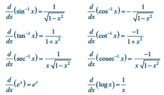
Following are some of the standard derivatives (in appropriate domains):
Logarithmic differentiation is a powerful technique to differentiate functions of the form f (x) = [u (x)]v(x) . Here both f (x) and u(x) need to be positive for this technique to make sense. v (x)
Rolle’s Theorem: If f : [a, b] → R is continuous on [a, b] and differentiable on (a, b) such that f (a) = f (b), then there exists some c in (a, b) such that f ′(c) = 0.
Mean Value Theorem: If f : [a, b] → R is continuous on [a, b] and differentiable on (a, b). Then there exists some c in (a, b) such that $f'(c) = \frac{f(b) - f(a)}{b - a}$
APPLICATION OF DERIVATIVES
If a quantity y varies with another quantity x, satisfying some rule y = f(x) then $\frac{dy}{dx}$ (or f(x)) represents the rate of change of y with respect to x and $\left [ \frac{dy}{dx} \right ]_{x = x_0}$ (or f '( $x_0$ ) ) represents the rate of change of y with respect to x at x = $x_0$
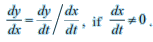
If two variables x and y are varying with respect to another variable t, i.e., if x = f(t) and y = g(t) , then by Chain Rule
A function f is said to be
(a) increasing on an interval (a, b) if x1 < x2 in (a,b) ⇒ f(x1) ≤ f(x2) for all x1 , x2 ∈ (a,b)
Alternatively, if f ′(x) ≥ 0 for each x in (a, b)
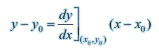
(b) decreasing on (a,b) if x1 < x2 in (a, b) ⇒ f (x 1 ) ≥ f (x 2 ) for all x 1 , x 2 ∈ (a,b)The equation of the tangent at (x0, y0) to the curve y = f (x) is given by
If $\frac{dy}{dx}$ does not exist at the point (x0,y0) then the tangent at this point is parallel to the y-axis and its equation is x = $x_0$
If tangent to a curve y = f (x) at x = $x_0$ is parallel to x-axis, then $\left [ \frac{dy}{dx} \right ]_{x = x_0}$ = 0
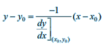
Equation of the normal to the curve y = f (x) at a point (x0,y0) is given by
If $\frac{dy}{dx}$ at the point (x0,y0) is zero, then equation of the normal is x = $x_0$
If $\frac{dy}{dx}$ at the point (x0,y0) does not exist , then then the normal is parallel to x-axis and its equation is y = $y_0$
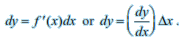
Let y = f (x), △ x be a small increment in x and △y be the increment in y corresponding to the increment in x, i.e., △y = f (x + △x) – f (x). Then dy given by below equaion and is a good approximation of △y when dx =△x is relatively small and we denote it by dy ≈ △y.
A point c in the domain of a function f at which either f ′(c) = 0 or f is not differentiable is called a critical point of f.
First Derivative Test Let f be a function defined on an open interval I. Let f be continuous at a critical point c in I. Then
If f ′(x) changes sign from positive to negative as x increases through c, i.e., if f ′(x) > 0 at every point sufficiently close to and to the left of c, and f ′(x) < 0 at every point sufficiently close to and to the right of c, then c is a point of local maxima.
If f ′(x) changes sign from negative to positive as x increases through c, i.e., if f ′(x) < 0 at every point sufficiently close to and to the left of c, and f ′(x) > 0 at every point sufficiently close to and to the right of c, then c is a point of local minima.
If f ′(x) does not change sign as x increases through c, then c is neither a point of local maxima nor a point of local minima. Infact, such a point is called point of inflexion.
Second Derivative Test Let f be a function defined on an interval I and c ∈ I. Let f be twice differentiable at c. Then
x = c is a point of local maxima if f ′(c) = 0 and f ″(c) < 0 The values f (c) is local maximum value of f .
x = c is a point of local minima if f ′(c) = 0 and f ″(c) > 0 In this case, f (c) is local minimum value of f .
The test fails if f ′(c) = 0 and f ″(c) = 0. In this case, we go back to the first derivative test and find whether c is a point of maxima, minima or a point of inflexion.
Working rule for finding absolute maxima and/or absolute minima
Step 1: Find all critical points of f in the interval, i.e., find points x where either f ′(x) = 0 or f is not differentiable.
Step 2:Take the end points of the interval
Step 3: At all these points (listed in Step 1 and 2), calculate the values of f .
Step 4:Identify the maximum and minimum values of f out of the values calculated in Step 3. This maximum value will be the absolute maximum value of f and the minimum value will be the absolute minimum value of f .
INTEGRALS
Integration is the inverse process of differentiation. In the differential calculus, we are given a function and we have to find the derivative or differential of this function, but in the integral calculus, we are to find a function whose differential is given. Thus, integration is a process which is the inverse of differentiation
Let $\frac{d}{dx} F(x) = f(x)$ . Then we write $\int$ f(x) dx = F(x) + C. These integrals are called indefinite integrals or general integrals, C is called constant of integration. All these integrals differ by a constant.
From the geometric point of view, an indefinite integral is collection of family of curves, each of which is obtained by translating one of the curves parallel to itself upwards or downwards along the y-axis.
Some properties of indefinite integrals are as follows:
$\int$ [f(x) + g(x) ] dx = $\int$ f(x) dx + $\int$ g(x) dx
For any real number k, $\int$ k f(x) dx = k $\int$ f(x) dx.
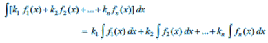
More generally, if f 1 , f 2 , f 3 , ... , f n are functions and k 1 , k 2 , ... ,k n are real numbers. Then
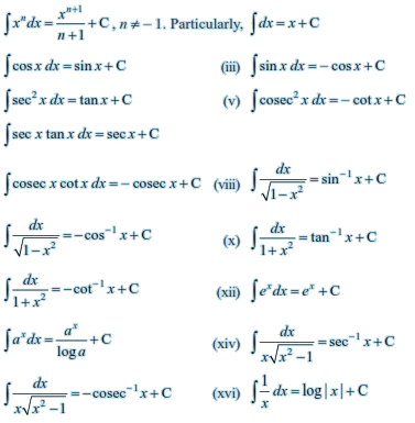
Some standard integrals
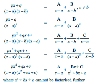
Integration by partial fractions
Integration by substitution
$\int$ tan x dx = log |sec x| + C
$\int$ cot x dx = log |sin x| + C
$\int$ sec x dx = log |sec x + tan x| + C
$\int$ cosec x dx = log |cosec x - cot x| + C
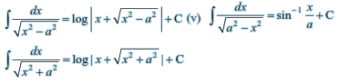
Integrals of some special functions
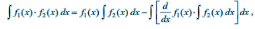
Integration by parts For given functions f 1 and f 2 , we have integral of the product of two functions = first function × integral of the second function – integral of {differential coefficient of the first function × integral of the second function}. Care must be taken in choosing the first function and the second function. Obviously, we must take that function as the second function whose integral is well known to us.
Some special types of integrals
Integrals of the types $\int \frac{px + q dx }{ax^2 + bx + c}$ or $\int \frac{px + q dx }{\sqrt{ax^2 + bx + c}}$ can be transformed into standard form by expressing $px + q = A\frac{d}{dx} (ax^2+bx+c)$ + B = A(2ax + b) + B , where A and B are determined by comparing coefficients on both sides.
We have defined $\int_{a}^{b} f(x) dx$ as the area of the region bounded by the curve y = f (x), a ≤ x ≤ b, the x-axis and the ordinates x = a and x = b. Let x be a given point in [a, b]. Then $\int_{x}^{a} f(x) dx$ represents the Area function A(x). This concept of area function leads to the Fundamental Theorems of Integral Calculus.
First fundamental theorem of integral calculus
Let the area function be defined by A(x) = $\int_{x}^{a} f(x) dx$ for all x ≥ a, where the function f is assumed to be continuous on [a, b]. Then A′ (x) = f (x) for all x ∈ [a, b]. f xdx
Second fundamental theorem of integral calculus
Let f be a continuous function of x defined on the closed interval [a, b] and let F be another function such that $\frac{d}{dx} F(x) = f(x)$ for all x in the domain of f, then $\int_{a}^{b} f(x) dx = [ F(x) + C ]_{a}^{b} = F(b) - F(a)$ This is called the definite integral of f over the range [a, b], where a and b are called the limits of integration, a being the lower limit and b the upper limit.