Preprocessing data
The sklearn.preprocessing package provides several common utility functions and transformer classes to change raw feature vectors into a representation that is more suitable for the downstream estimators.
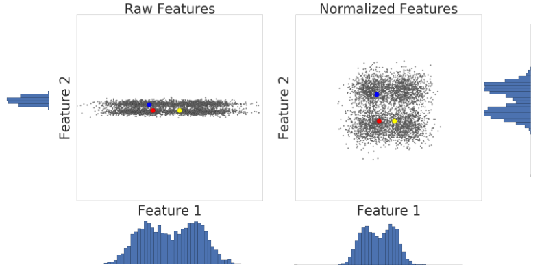
In general, learning algorithms benefit from standardization of the data set. If some outliers are present in the set, robust scalers or transformers are more appropriate.
The behaviors of the different scalers, transformers, and normalizers on a dataset containing marginal outliers is highlighted in Compare the effect of different scalers on data with outliers.
The Python tutorials are written as Jupyter notebooks and run directly in Google Colab—a hosted notebook environment that requires no setup. Click the Run in Google Colab button.
Colab link - Open colab
Standardization, or mean removal and variance scaling
Standardization of datasets is a common requirement for many machine learning estimators implemented in scikit-learn; they might behave badly if the individual features do not more or less look like standard normally distributed data: Gaussian with zero mean and unit variance.
In practice we often ignore the shape of the distribution and just transform the data to center it by removing the mean value of each feature, then scale it by dividing non-constant features by their standard deviation.
For instance, many elements used in the objective function of a learning algorithm (such as the RBF kernel of Support Vector Machines or the l1 and l2 regularizers of linear models) assume that all features are centered around zero and have variance in the same order.
If a feature has a variance that is orders of magnitude larger than others, it might dominate the objective function and make the estimator unable to learn from other features correctly as expected.
The function scale provides a quick and easy way to perform this operation on a single array-like dataset:
from sklearn import preprocessing
import numpy as np
X_train = np.array([[ 1., -1.,  2.],
                    [ 2.,  0.,  0.],
                    [ 0.,  1., -1.]])
X_scaled = preprocessing.scale(X_train)

X_scaled
Scaled data has zero mean and unit variance
X_scaled.mean(axis=0)

X_scaled.std(axis=0)
StandardScaler
scaler = preprocessing.StandardScaler().fit(X_train)
scaler

scaler.mean_

scaler.scale_

scaler.transform(X_train)
The scaler instance can then be used on new data to transform it the same way it did on the training set:
X_test = [[-1., 1., 0.]]
scaler.transform(X_test)
Scaling features to a range
An alternative standardization is scaling features to lie between a given minimum and maximum value, often between zero and one, or so that the maximum absolute value of each feature is scaled to unit size.
This can be achieved using MinMaxScaler or MaxAbsScaler, respectively.
The motivation to use this scaling include robustness to very small standard deviations of features and preserving zero entries in sparse data.
X_train = np.array([[ 1., -1.,  2.],
                    [ 2.,  0.,  0.],
                    [ 0.,  1., -1.]])

min_max_scaler = preprocessing.MinMaxScaler()
X_train_minmax = min_max_scaler.fit_transform(X_train)
X_train_minmax
The same instance of the transformer can then be applied to some new test data unseen during the fit call: the same scaling and shifting operations will be applied to be consistent with the transformation performed on the train data:
X_test = np.array([[-3., -1.,  4.]])
X_test_minmax = min_max_scaler.transform(X_test)
X_test_minmax
MaxAbsScaler works in a very similar fashion, but scales in a way that the training data lies within the range [-1, 1] by dividing through the largest maximum value in each feature. It is meant for data that is already centered at zero or sparse data.
X_train = np.array([[ 1., -1.,  2.],
                    [ 2.,  0.,  0.],
                    [ 0.,  1., -1.]])

max_abs_scaler = preprocessing.MaxAbsScaler()

X_train_maxabs = max_abs_scaler.fit_transform(X_train)

X_train_maxabs

X_test = np.array([[ -3., -1.,  4.]])

X_test_maxabs = max_abs_scaler.transform(X_test)

X_test_maxabs

max_abs_scaler.scale_
RobustScaler Scale features using statistics that are robust to outliers.
This Scaler removes the median and scales the data according to the quantile range (defaults to IQR: Interquartile Range). The IQR is the range between the 1st quartile (25th quantile) and the 3rd quartile (75th quantile).
Centering and scaling happen independently on each feature by computing the relevant statistics on the samples in the training set. Median and interquartile range are then stored to be used on later data using the transform method.
Standardization of a dataset is a common requirement for many machine learning estimators. Typically this is done by removing the mean and scaling to unit variance. However, outliers can often influence the sample mean / variance in a negative way. In such cases, the median and the interquartile range often give better results.
from sklearn.preprocessing import RobustScaler
X = [[ 1., -2.,  2.],
     [ -2.,  1.,  3.],
     [ 4.,  1., -2.]]

transformer = RobustScaler().fit(X)

transformer

transformer.transform(X)
Preparation of data
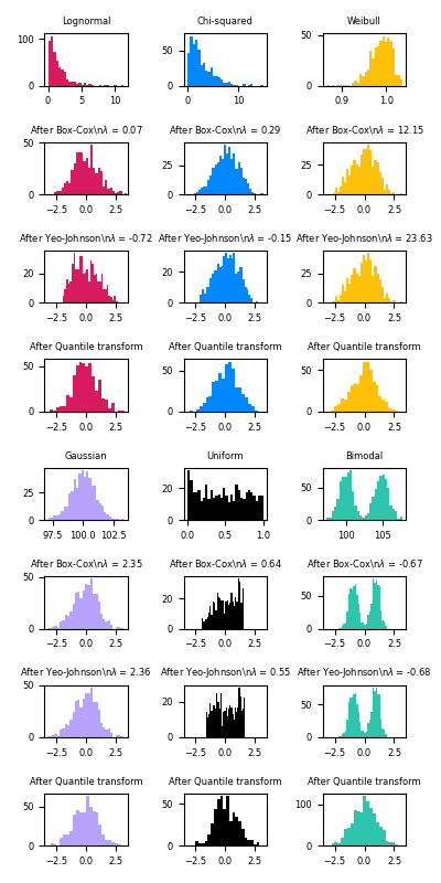
1. As a rule of thumb, to create quantiles, you should have at least examples 10n. If you don't have enough data, stick to normalization.
2. Log transform data if it conforms to a power law
3. Normalize data if it conforms to gaussian distribution
Mapping to a Uniform distribution QuantileTransformer and quantile_transform provide a non-parametric transformation to map the data to a uniform distribution with values between 0 and 1
from sklearn.datasets import load_iris
from sklearn.model_selection import train_test_split
X, y = load_iris(return_X_y=True)
X_train, X_test, y_train, y_test = train_test_split(X, y, random_state=0)
quantile_transformer = preprocessing.QuantileTransformer(random_state=0)
X_train_trans = quantile_transformer.fit_transform(X_train)
X_test_trans = quantile_transformer.transform(X_test)
Mapping to a Gaussian distribution In many modeling scenarios, normality of the features in a dataset is desirable. Power transforms are a family of parametric, monotonic transformations that aim to map data from any distribution to as close to a Gaussian distribution as possible in order to stabilize variance and minimize skewness.
PowerTransformer currently provides two such power transformations, the Yeo-Johnson transform and the Box-Cox transform.
Box-Cox can only be applied to strictly positive data
pt = preprocessing.PowerTransformer(method='box-cox', standardize=False)
X_lognormal = np.random.RandomState(616).lognormal(size=(3, 3))
X_lognormal

pt.fit_transform(X_lognormal)
It is also possible to map data to a normal distribution using QuantileTransformer by setting output_distribution='normal'. Using the earlier example with the iris dataset
quantile_transformer = preprocessing.QuantileTransformer(
     output_distribution='normal', random_state=0)
X_trans = quantile_transformer.fit_transform(X)
quantile_transformer.quantiles_
Normalization
X = [[ 1., -1.,  2.],
     [ 2.,  0.,  0.],
     [ 0.,  1., -1.]]

X_normalized = preprocessing.normalize(X, norm='l2')

X_normalized
The preprocessing module further provides a utility class Normalizer that implements the same operation
normalizer = preprocessing.Normalizer().fit(X)  # fit does nothing
normalizer
Encoding categorical features Often features are not given as continuous values but categorical.
For example a person could have features ["male", "female"], ["from Europe", "from US", "from Asia"], ["uses Firefox", "uses Chrome", "uses Safari", "uses Internet Explorer"].
Such features can be efficiently coded as integers, for instance ["male", "from US", "uses Internet Explorer"] could be expressed as [0, 1, 3] while ["female", "from Asia", "uses Chrome"] would be [1, 2, 1].
Such integer representation can, however, not be used directly with all scikit-learn estimators
enc = preprocessing.OrdinalEncoder()
X = [['male', 'from US', 'uses Safari'], ['female', 'from Europe', 'uses Firefox']]
enc.fit(X)
enc.transform([['female', 'from US', 'uses Safari']])
Another possibility to convert categorical features to features that can be used with scikit-learn estimators is to use a one-of-K, also known as one-hot or dummy encoding. This type of encoding can be obtained with the OneHotEncoder,
enc = preprocessing.OneHotEncoder()
X = [['male', 'from US', 'uses Safari'], ['female', 'from Europe', 'uses Firefox']]
enc.fit(X)
enc.transform([['female', 'from US', 'uses Safari'],
               ['male', 'from Europe', 'uses Safari']]).toarray()
By default, the values each feature can take is inferred automatically from the dataset and can be found in the categories_ attribute
enc.categories_
It is possible to specify this explicitly using the parameter categories. There are two genders, four possible continents and four web browsers in our dataset:
genders = ['female', 'male']
locations = ['from Africa', 'from Asia', 'from Europe', 'from US']
browsers = ['uses Chrome', 'uses Firefox', 'uses IE', 'uses Safari']
enc = preprocessing.OneHotEncoder(categories=[genders, locations, browsers])

X = [['male', 'from US', 'uses Safari'], ['female', 'from Europe', 'uses Firefox']]
enc.fit(X)

enc.transform([['female', 'from Asia', 'uses Chrome']]).toarray()
If there is a possibility that the training data might have missing categorical features, it can often be better to specify handle_unknown='ignore' instead of setting the categories manually as above.
When handle_unknown='ignore' is specified and unknown categories are encountered during transform, no error will be raised but the resulting one-hot encoded columns for this feature will be all zeros (handle_unknown='ignore' is only supported for one-hot encoding)
enc = preprocessing.OneHotEncoder(handle_unknown='ignore')
X = [['male', 'from US', 'uses Safari'], ['female', 'from Europe', 'uses Firefox']]
enc.fit(X)
enc.transform([['female', 'from Asia', 'uses Chrome']]).toarray()
One might want to drop one of the two columns only for features with 2 categories. In this case, you can set the parameter drop='if_binary'
X = [['male', 'US', 'Safari'],
     ['female', 'Europe', 'Firefox'],
     ['female', 'Asia', 'Chrome']]

drop_enc = preprocessing.OneHotEncoder(drop='if_binary').fit(X)

drop_enc.categories_

drop_enc.transform(X).toarray()
Simple Imputer - Univariate feature imputation The SimpleImputer class provides basic strategies for imputing missing values.
Missing values can be imputed with a provided constant value, or using the statistics (mean, median or most frequent) of each column in which the missing values are located. This class also allows for different missing values encodings.
The following snippet demonstrates how to replace missing values, encoded as np.nan, using the mean value of the columns (axis 0) that contain the missing values:
import numpy as np
from sklearn.impute import SimpleImputer
imp = SimpleImputer(missing_values=np.nan, strategy='mean')
imp.fit([[1, 2], [np.nan, 3], [7, 6]])
X = [[np.nan, 2], [6, np.nan], [7, 6]]
print(imp.transform(X))
The SimpleImputer class also supports categorical data represented as string values or pandas categoricals when using the 'most_frequent' or 'constant' strategy:
import pandas as pd
df = pd.DataFrame([["a", "x"],
                   [np.nan, "y"],
                   ["a", np.nan],
                   ["b", "y"]], dtype="category")

imp = SimpleImputer(strategy="most_frequent")
print(imp.fit_transform(df))
Multivariate feature imputation A more sophisticated approach is to use the IterativeImputer class, which models each feature with missing values as a function of other features, and uses that estimate for imputation.
It does so in an iterated round-robin fashion: at each step, a feature column is designated as output y and the other feature columns are treated as inputs X.
A regressor is fit on (X, y) for known y. Then, the regressor is used to predict the missing values of y.
This is done for each feature in an iterative fashion, and then is repeated for max_iter imputation rounds.
The results of the final imputation round are returned.
import numpy as np
from sklearn.experimental import enable_iterative_imputer
from sklearn.impute import IterativeImputer
imp = IterativeImputer(max_iter=10, random_state=0)


imp.fit([[1, 2], [3, 6], [4, 8], [np.nan, 3], [7, np.nan]])

X_test = [[np.nan, 2], [6, np.nan], [np.nan, 6]]

print(np.round(imp.transform(X_test)))
Nearest neighbors imputation The KNNImputer class provides imputation for filling in missing values using the k-Nearest Neighbors approach.
By default, a euclidean distance metric that supports missing values, nan_euclidean_distances, is used to find the nearest neighbors.
Each missing feature is imputed using values from n_neighbors nearest neighbors that have a value for the feature. The feature of the neighbors are averaged uniformly or weighted by distance to each neighbor.
If a sample has more than one feature missing, then the neighbors for that sample can be different depending on the particular feature being imputed.
When the number of available neighbors is less than n_neighbors and there are no defined distances to the training set, the training set average for that feature is used during imputation.
If there is at least one neighbor with a defined distance, the weighted or unweighted average of the remaining neighbors will be used during imputation. If a feature is always missing in training, it is removed during transform. For more information on the methodology
The following snippet demonstrates how to replace missing values, encoded as np.nan, using the mean feature value of the two nearest neighbors of samples with missing values:
import numpy as np
from sklearn.impute import KNNImputer
nan = np.nan
X = [[1, 2, nan], [3, 4, 3], [nan, 6, 5], [8, 8, 7]]
imputer = KNNImputer(n_neighbors=2, weights="uniform")
imputer.fit_transform(X)