Python Collections - 1D Numpy Array
The Python tutorials are written as Jupyter notebooks and run directly in Google Colab—a hosted notebook environment that requires no setup. Click the Run in Google Colab button.
Colab link - Open colab
Preparation
# Import the libraries

import time
import sys
import numpy as np

import matplotlib.pyplot as plt
%matplotlib inline

# Plotting functions

def Plotvec1(u, z, v):

    ax = plt.axes()
    ax.arrow(0, 0, *u, head_width=0.05, color='r', head_length=0.1)
    plt.text(*(u + 0.1), 'u')

    ax.arrow(0, 0, *v, head_width=0.05, color='b', head_length=0.1)
    plt.text(*(v + 0.1), 'v')
    ax.arrow(0, 0, *z, head_width=0.05, head_length=0.1)
    plt.text(*(z + 0.1), 'z')
    plt.ylim(-2, 2)
    plt.xlim(-2, 2)

def Plotvec2(a,b):
    ax = plt.axes()
    ax.arrow(0, 0, *a, head_width=0.05, color ='r', head_length=0.1)
    plt.text(*(a + 0.1), 'a')
    ax.arrow(0, 0, *b, head_width=0.05, color ='b', head_length=0.1)
    plt.text(*(b + 0.1), 'b')
    plt.ylim(-2, 2)
    plt.xlim(-2, 2)
Create a Python List as follows:
# Create a python list

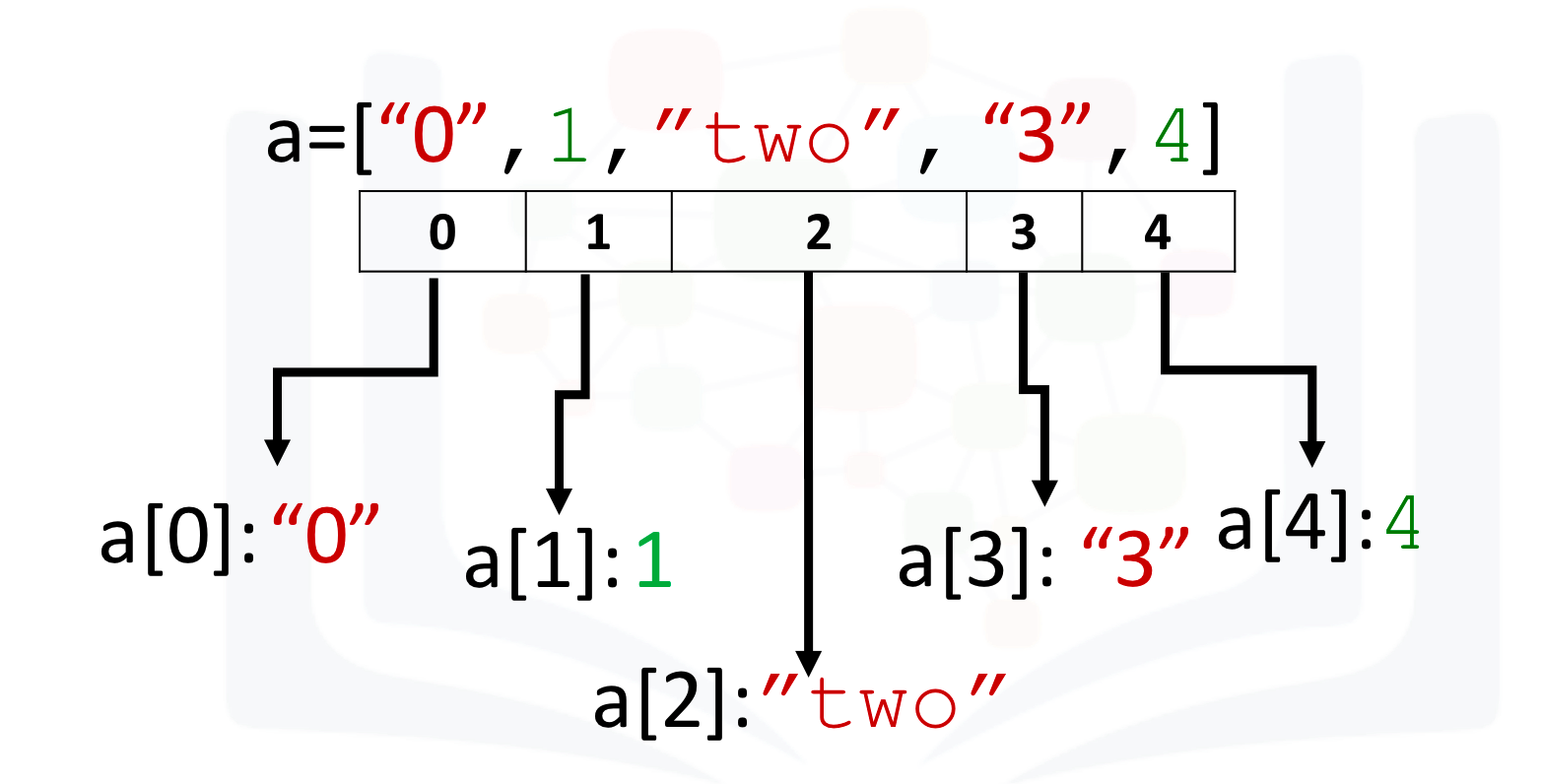
a = ["0", 1, "two", "3", 4]
We can access the data via an index:

We can access each element using a square bracket as follows:
# Print each element

print("a[0]:", a[0])
print("a[1]:", a[1])
print("a[2]:", a[2])
print("a[3]:", a[3])
print("a[4]:", a[4])
What is Numpy?
A numpy array is similar to a list. It's usually fixed in size and each element is of the same type. We can cast a list to a numpy array by first importing numpy:
# import numpy library

import numpy as np
We then cast the list as follows:
# Create a numpy array

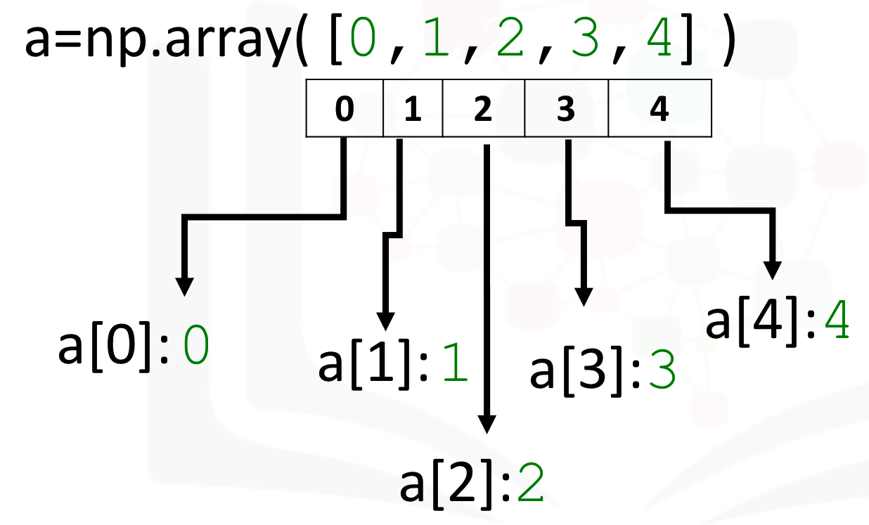
a = np.array([0, 1, 2, 3, 4])
a
Each element is of the same type, in this case integers:

As with lists, we can access each element via a square bracket:
# Print each element

print("a[0]:", a[0])
print("a[1]:", a[1])
print("a[2]:", a[2])
print("a[3]:", a[3])
print("a[4]:", a[4])
Type
If we check the type of the array we get numpy.ndarray:
# Check the type of the array

type(a)
As numpy arrays contain data of the same type, we can use the attribute "dtype" to obtain the Data-type of the array’s elements. In this case a 64-bit integer:
# Check the type of the values stored in numpy array

a.dtype
We can create a numpy array with real numbers:
# Create a numpy array

b = np.array([3.1, 11.02, 6.2, 213.2, 5.2])
When we check the type of the array we get numpy.ndarray:
# Check the type of array

type(b)
If we examine the attribute dtype we see float 64, as the elements are not integers:
# Check the value type

b.dtype
Assign value
We can change the value of the array, consider the array c:
# Create numpy array

c = np.array([20, 1, 2, 3, 4])
c
We can change the first element of the array to 100 as follows:
# Assign the first element to 100

c[0] = 100
c
We can change the 5th element of the array to 0 as follows:
# Assign the 5th element to 0

c[4] = 0
c
Slicing
Like lists, we can slice the numpy array, and we can select the elements from 1 to 3 and assign it to a new numpy array d as follows:
# Slicing the numpy array

d = c[1:4]
d
We can assign the corresponding indexes to new values as follows:
# Set the fourth element and fifth element to 300 and 400

c[3:5] = 300, 400
c
Assign Value with List
Similarly, we can use a list to select a specific index. The list ' select ' contains several values:
# Create the index list

select = [0, 2, 3]
We can use the list as an argument in the brackets. The output is the elements corresponding to the particular index:
# Use List to select elements

d = c[select]
d
We can assign the specified elements to a new value. For example, we can assign the values to 100 000 as follows:
# Assign the specified elements to new value

c[select] = 100000
c
Other Attributes
Let's review some basic array attributes using the array a:
# Create a numpy array

a = np.array([0, 1, 2, 3, 4])
a
The attribute size is the number of elements in the array:
# Get the size of numpy array

a.size
The next two attributes will make more sense when we get to higher dimensions but let's review them. The attribute ndim represents the number of array dimensions or the rank of the array, in this case, one:
# Get the number of dimensions of numpy array

a.ndim
The attribute shape is a tuple of integers indicating the size of the array in each dimension:
# Get the shape/size of numpy array

a.shape

# Create a numpy array

a = np.array([1, -1, 1, -1])

# Get the mean of numpy array

mean = a.mean()
mean

# Get the standard deviation of numpy array

standard_deviation=a.std()
standard_deviation

# Create a numpy array

b = np.array([-1, 2, 3, 4, 5])
b

# Get the biggest value in the numpy array

max_b = b.max()
max_b

# Get the smallest value in the numpy array

min_b = b.min()
min_b
Numpy Array Operations
Array Addition
Consider the numpy array u:
u = np.array([1, 0])
u
Consider the numpy array v:
v = np.array([0, 1])
v
We can add the two arrays and assign it to z:
# Numpy Array Addition

z = u + v
z
The operation is equivalent to vector addition:
# Plot numpy arrays

Plotvec1(u, z, v)
Array Multiplication
Consider the vector numpy array y:
# Create a numpy array

y = np.array([1, 2])
y
We can multiply every element in the array by 2:
# Numpy Array Multiplication

z = 2 * y
z
This is equivalent to multiplying a vector by a scaler:
Product of Two Numpy Arrays
Consider the following array u:
# Create a numpy array

u = np.array([1, 2])
u
Consider the following array v:
# Create a numpy array

v = np.array([3, 2])
v
The product of the two numpy arrays u and v is given by:
# Calculate the production of two numpy arrays

z = u * v
z
Dot Product
The dot product of the two numpy arrays u and v is given by:
# Calculate the dot product

np.dot(u, v)
Adding Constant to a Numpy Array
Consider the following array:
# Create a constant to numpy array

u = np.array([1, 2, 3, -1])
u
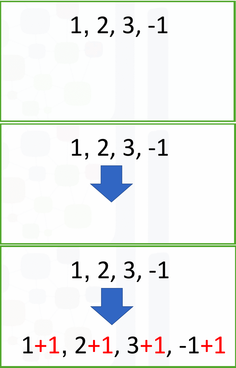
Adding the constant 1 to each element in the array:
# Add the constant to array

u + 1
The process is summarised in the following animation:

Mathematical Functions
We can access the value of pie in numpy as follows :
# The value of pie

np.pi
We can create the following numpy array in Radians:
# Create the numpy array in radians

x = np.array([0, np.pi/2 , np.pi])
We can apply the function sin to the array x and assign the values to the array y; this applies the sine function to each element in the array:
# Calculate the sin of each elements

y = np.sin(x)
y
Linspace
A useful function for plotting mathematical functions is "linespace". Linespace returns evenly spaced numbers over a specified interval. We specify the starting point of the sequence and the ending point of the sequence. The parameter "num" indicates the Number of samples to generate, in this case 5:
# Makeup a numpy array within [-2, 2] and 5 elements

np.linspace(-2, 2, num=5)
If we change the parameter num to 9, we get 9 evenly spaced numbers over the interval from -2 to 2:
# Makeup a numpy array within [-2, 2] and 9 elements

np.linspace(-2, 2, num=9)
We can use the function line space to generate 100 evenly spaced samples from the interval 0 to 2π:
# Makeup a numpy array within [0, 2π] and 100 elements

x = np.linspace(0, 2*np.pi, num=100)
We can apply the sine function to each element in the array x and assign it to the array y:
# Calculate the sine of x list

y = np.sin(x)

# Plot the result

plt.plot(x, y)