Python Collections - 2D Numpy Array
The Python tutorials are written as Jupyter notebooks and run directly in Google Colab—a hosted notebook environment that requires no setup. Click the Run in Google Colab button.
Colab link - Open colab
Create a 2D Numpy Array
# Import the libraries

import numpy as np
import matplotlib.pyplot as plt
Consider the list a, the list contains three nested lists **each of equal size**.
# Create a list

a = [[11, 12, 13], [21, 22, 23], [31, 32, 33]]
a
We can cast the list to a Numpy Array as follow
# Convert list to Numpy Array
# Every element is the same type

A = np.array(a)
A
We can use the attribute ndim to obtain the number of axes or dimensions referred to as the rank.
# Show the numpy array dimensions

A.ndim
Attribute shape returns a tuple corresponding to the size or number of each dimension.
# Show the numpy array shape

A.shape
The total number of elements in the array is given by the attribute size.
# Show the numpy array size

A.size
Accessing different elements of a Numpy Array
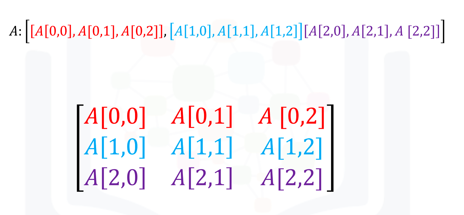
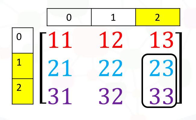
We can use rectangular brackets to access the different elements of the array. The correspondence between the rectangular brackets and the list and the rectangular representation is shown in the following figure for a 3x3 array:
We can access the 2nd-row 3rd column as shown in the following figure:
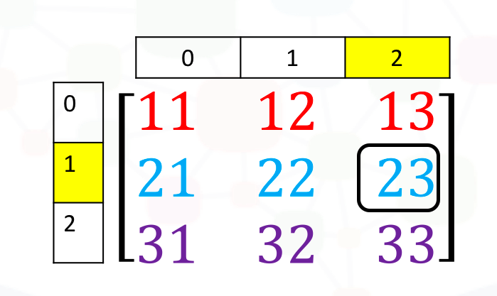
We simply use the square brackets and the indices corresponding to the element we would like:
# Access the element on the second row and third column

A[1, 2]
We can also use the following notation to obtain the elements:
# Access the element on the second row and third column

A[1][2]
Consider the elements shown in the following figure
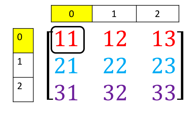
We can access the element as follows
# Access the element on the first row and first column

A[0][0]
We can also use slicing in numpy arrays. Consider the following figure. We would like to obtain the first two columns in the first row
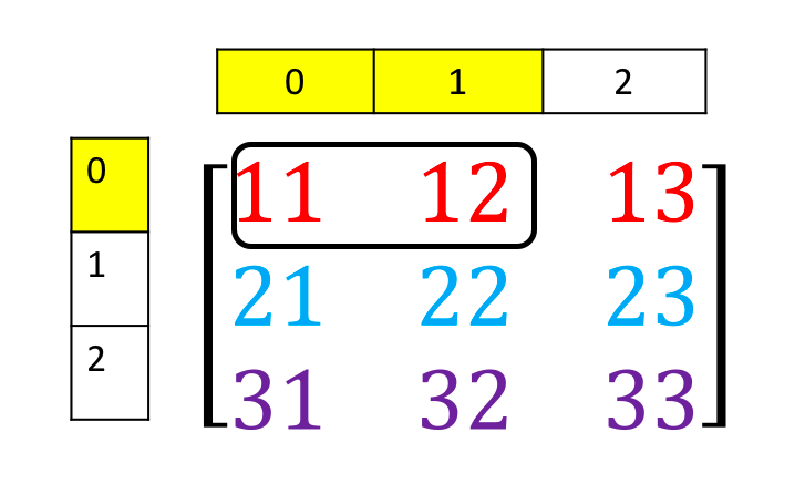
This can be done with the following syntax
# Access the element on the first row and first and second columns

A[0][0:2]
Similarly, we can obtain the first two rows of the 3rd column as follows:
# Access the element on the first and second rows and third column

A[0:2, 2]
Corresponding to the following figure:
Basic Operations
We can also add arrays. The process is identical to matrix addition. Matrix addition of X and Y is shown in the following figure:
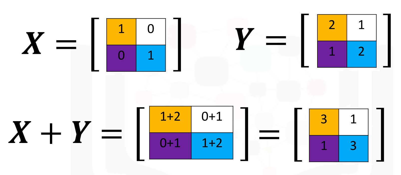
The numpy array is given by X and Y
# Create a numpy array X

X = np.array([[1, 0], [0, 1]])
X

# Create a numpy array Y

Y = np.array([[2, 1], [1, 2]])
Y
We can add the numpy arrays as follows.
# Add X and Y

Z = X + Y
Z
Multiplying a numpy array by a scaler is identical to multiplying a matrix by a scaler. If we multiply the matrix Y by the scaler 2, we simply multiply every element in the matrix by 2 as shown in the figure.
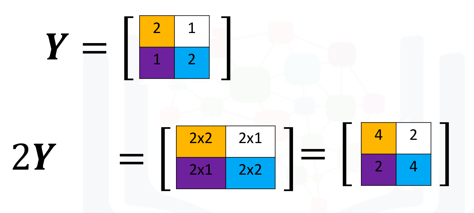
We can perform the same operation in numpy as follows
# Create a numpy array Y

Y = np.array([[2, 1], [1, 2]])
Y

# Multiply Y with 2

Z = 2 * Y
Z
Multiplication of two arrays corresponds to an element-wise product or Hadamard product. Consider matrix X and Y. The Hadamard product corresponds to multiplying each of the elements in the same position, i.e. multiplying elements contained in the same color boxes together. The result is a new matrix that is the same size as matrix Y or X, as shown in the following figure.
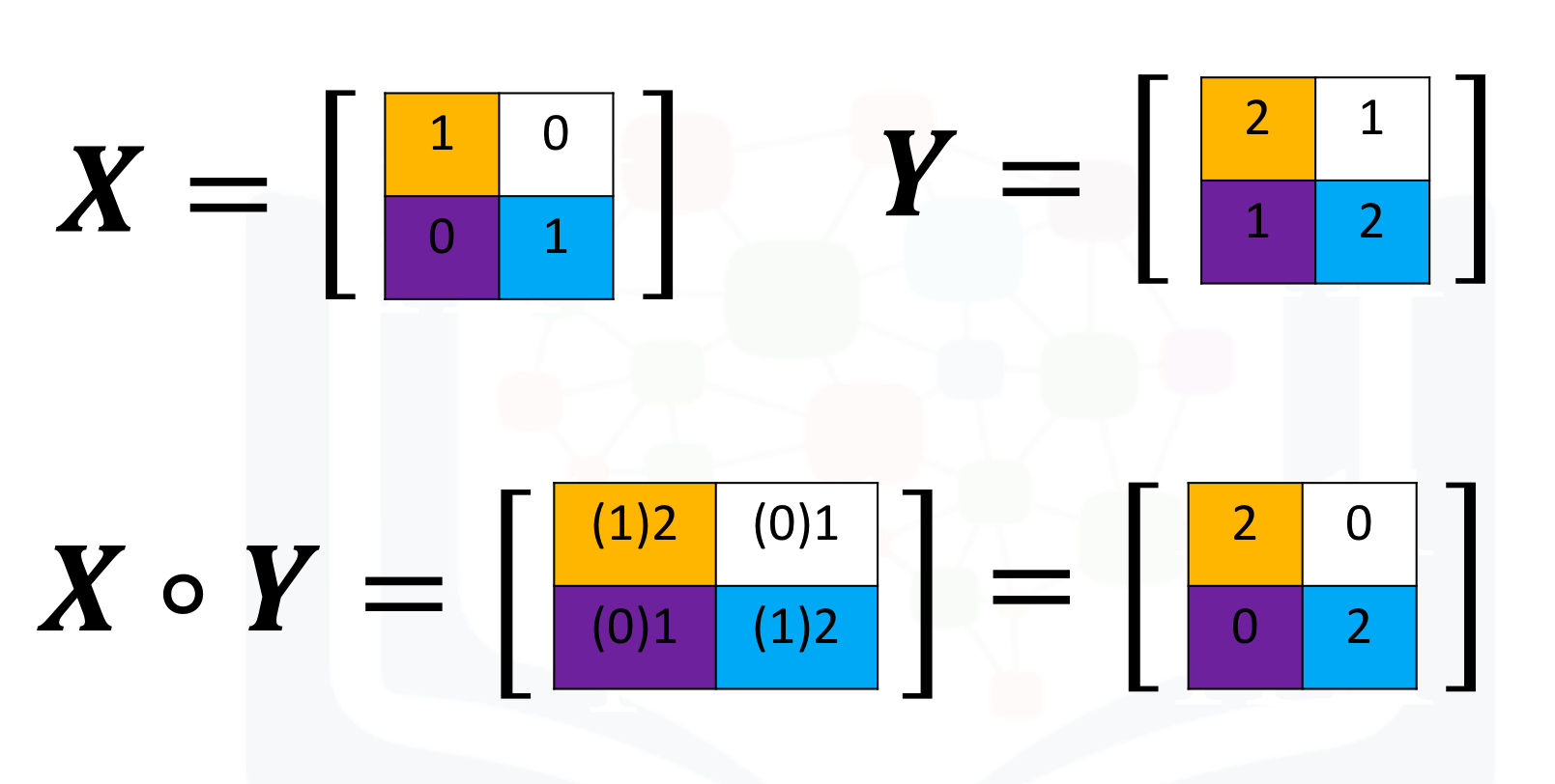
We can perform element-wise product of the array X and Y as follows:
# Create a numpy array Y

Y = np.array([[2, 1], [1, 2]])
Y

# Create a numpy array X

X = np.array([[1, 0], [0, 1]])
X

# Multiply X with Y

Z = X * Y
Z
We can also perform matrix multiplication with the numpy arrays A and B as follows:
First, we define matrix A and B:
# Create a matrix A

A = np.array([[0, 1, 1], [1, 0, 1]])
A

# Create a matrix B

B = np.array([[1, 1], [1, 1], [-1, 1]])
B
We use the numpy function dot to multiply the arrays together.
# Calculate the dot product

Z = np.dot(A,B)
Z

# Calculate the sine of Z

np.sin(Z)
We use the numpy attribute T to calculate the transposed matrix
# Create a matrix C

C = np.array([[1,1],[2,2],[3,3]])
C

# Get the transposed of C

C.T